Chapter 9 - Decision Trees and Ensemble Methods

Another field of models in classical supervised machine learning. This lecture will cover decision trees and ensemble methods. So, what are decision trees and why would we want to use these models? Consider the following dataset:

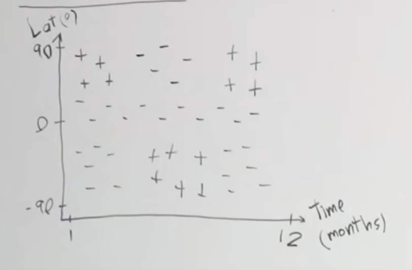
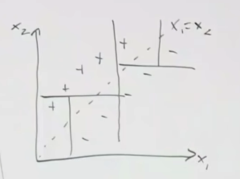
Say this is a plot of when certain areas in the world are cold enough for skiing. 90 degrees in latitude is the north pole, and the other is the south pole and southern hemisphere. So, we see patches of data that we want to build a model that can isolate the positives from the negatives. With existing knowledge, maybe we build some sort of neural network or find a kernel function to lift this into a higher space, and then build an SVM. We introduce a new category of models called decision trees, which will handle these patches of data.

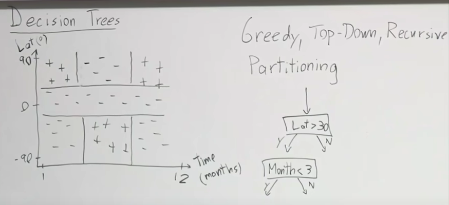
Decision Trees

Decision trees are a more natural way of accomplishing this. Decision trees aim to split the region, and to do so, uses a greedy top-down recursive partitioning.

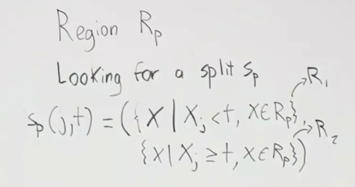
So, we want these functions that split the region → How to choose splits? Define $L (R)$ : Loss on R given C classes, define $\overset{p}{^}_{C}$ to be the proportion of examples in R that are of class C. We also define $L_{mi sc l a ss} = 1 - ma x_{c} \overset{p}{^}_{C}$ . In the above, we are splitting the parent region into children regions, R1 and R2. The goal is to reduce the loss as much as possible: max $L (R_{p}) - (L (R_{1}) + L (R_{2}))$ which is difference between parent loss and children loss. However this way of thinking has issues. To illustrate this, consider the following example:

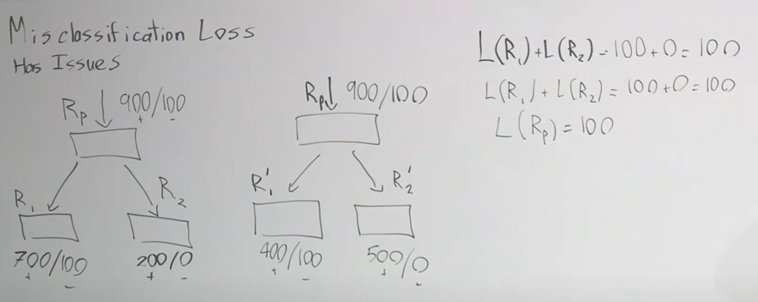
First of all, the loss metric for the 2 situations is the same, but most would agree that the right is more preferable as we separating more definite positives (group with no misclassifications has more positives inside it). But, if we look at the loss of the parent function, it is the same as the ones from the children. So, did nothing improve? This shows that this loss metric is not sensitive enough and not very informative. Instead, what we can do is to define a cross-entropy loss: $L_{cross} = - \sum_{c} \hat{P}_{c} lo g_{2} \hat{P}_{c}$ .

Are there any limits we should impose? Yes. If the we allow the decision tree to grow arbitrarily large, we could end up having a separate region for every data point that we have. That would vastly overfit. One thing we are interested in doing is regularizing these high variance models. Generally, a couple of heuristics can be followed:

Min leaf size → stop splitting when this is reached
Max depth size
Max number of nodes
Minimum decrease in loss (generally not a good idea. Sometimes one question does not tell us much, but in combination with others, does. Good example is the first image of the data points. First horizontal line does not tell us much, and would have very small decrease in loss. But when we add on questions that draw vertical lines, it becomes much more informative. This method comes at the risk of pre-mature stopping in our algorithm).

However, there are a number of downsides to decision trees: they don’t have additive structure.

→ No Additive Structure

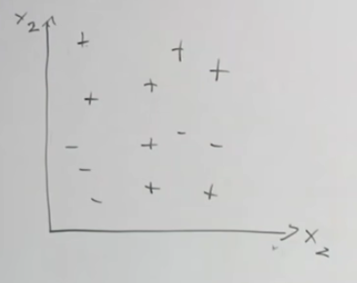
Data like this, where something like logistic regression would be able to model very easily, is a struggle for decision trees. We would need to ask a lot of questions to even come close to approximating this line. So, now let’s talk about ensembling.

Ensembling

Model ensembling combines the predictions from multiple models together. Traditionally this is done by running each model on some inputs separately and then combining the predictions. However, if you’re running models with the same architecture, then it may be possible to combine them together using specific library functionality. The main idea behind ensemble learning is that by combining the predictions of multiple models, the ensemble can reduce variance, bias, or improve predictions.

There are several types of ensemble methods, each with its unique approach to combining models:

Bagging (Bootstrap Aggregating):
1. Example: Random Forest.
2. How it works: Multiple versions of a predictor are trained on different subsets of the data created by randomly sampling with replacement (bootstrapping). The final prediction is typically made by averaging the predictions (for regression) or majority voting (for classification) of all the predictors.
Boosting:
1. Example: AdaBoost, Gradient Boosting Machines (GBM), XGBoost.
2. How it works: Models are trained sequentially, each trying to correct the errors of the previous one. The final model is a weighted sum of the individual models, where more weight is given to models that perform better.
Stacking (Stacked Generalization):
1. How it works: Different types of models (base models) are trained on the same dataset. A new model (meta-model) is then trained to combine the predictions of the base models. The meta-model aims to learn the best way to combine these predictions to make a final prediction.
Voting:
1. How it works: Multiple models are trained and their predictions are combined by voting (for classification) or averaging (for regression). There are two types of voting:
  1. Hard Voting: Each base model votes for a class label and the class with the majority vote is the final prediction.
  2. Soft Voting: Each base model outputs the probability of each class and the class with the highest summed probability is the final prediction.

Advantages of Ensemble Learning:

Improved Accuracy: By combining the strengths of multiple models, ensembles often achieve higher accuracy than individual models.
Robustness: Ensembles are less likely to overfit the training data compared to individual models.
Flexibility: They can be used with different types of base models and are adaptable to various types of data and problems.

Disadvantages of Ensemble Learning:

Complexity: Ensembles are more complex and computationally intensive than individual models.
Interpretability: It can be harder to interpret the results of an ensemble compared to a single model.
Resource-Intensive: Training multiple models and combining their predictions requires more computational resources and time.

There are a couple of ways of doing ensemble learning, and likely, something we want to do for the final project. This is what people on Kaggle will do when they really want to maximize the accuracy of their models, so definition implement this for the final project

Raphael Townshend ~ “Take a NN, or Transformer, or SVM, average them all together and generally, yields good results”, but is much more time consuming, as we are spending time implementing each of these algorithms

So, in summary, we have:

Different algorithms
Different training sets But its unrealistic to just say “go find more data to train on : /“. The above is an example, but in this lecture, we will focus on 2 types: bagging, which is trying to approximate having different training sets, and boosting. We’ll use decision trees to talk a lot about these models, and so for bagging, we’ll take a look at random forests, and for boosting, we’ll see Adaboost, XGBoost. So, boosting and bagging are more efficient methods of trying to achieve what the first 2 ensemble methods were, due to their downsides (complexity and infeasibility).

Bagging

Bagging really stands for bootstrap aggregation. Bootstrapping is a technique used in statistics, to measure the uncertainty in your estimation. Say we have some true population $P$ , we define a training set to be some sample of the true population $S \sim P$ . So, ideally, what we want to do is keep drawing training sets $S_{i}$ , and train models on each of those separately, Unfortunately, we often don’t have the time for that. So, what we do instead, we bootstrap: assume the population is the training sample, and then, we draw new samples from $S$ , and we call these bootstrap samples $Z \sim S$ , where we draw these samples with replacement (important). We want to aggregate the bootstrap samples, so at a high level, we are train separate models on each of the bootstrap samples, and average their outputs.

B oo t s t r a pS am pl es (Z_{1}, \dots, \overset{ˉ}{Z}_{M}) T r ainm o d e l (G_{m}) o n (\overset{ˉ}{Z}_{m}) G (m) = \frac{1}{M} m = 1 \sum M G_{m} (x)

→ Bias-variance Analysis

Bias-Variance Tradeoff: This is a fundamental concept in machine learning that describes the tradeoff between bias (error due to overly simplistic models) and variance (error due to models being too complex and sensitive to training data)
Equation: The equation below is a variance decomposition formula which is often used to understand the components contributing to the variance of an estimator.

Var (\overset{ˉ}{X}) = ρ σ^{2} + \frac{1 - ρ}{M} σ^{2} Bootstrapping is driving down p

To see derivation of this, visit https://www.youtube.com/watch?v=wr9gUr-eWdA&t=82s&ab_channel=StanfordOnline at time-stamp 53:51

$M$ is the number of bootstrap samples and $ρ$ proportion of correctly classified. Bootstrapping de-correlating the models we have trained, and thereby driving down the $ρ$ , the proportion of variance due to the bias of the model. In the case of Decision trees, they are prone to high variance because small changes in the training data can result in significantly different trees. Bagging helps reduce the variance of decision trees by averaging multiple trees trained on different bootstrap samples of the training data. So, by taking more and more bootstrap samples, we increase $M$ and decrease $ρ$ without the risk of overfitting as well. It’s worth noting that bias is increased as a result of taking these bootstrapped samples.

DTs + Bagging

DT are high variance and low bias. This is why they are a good fit for bagging, as bagging decreases the variance of the model for a slight increase in bias. Since most of the loss of DTs were coming from the high variance, bagging reduces this and is an ideal fit. This is basically the idea of Random Forest, with the only difference being, it introduces even more randomness in each decision tree.

Extension of Bagging: Random forests extend the idea of bagging by adding an additional layer of randomness to the model:

Method:
- Like bagging, multiple subsets of the training data are created using bootstrapping.
- However, when constructing each tree, instead of considering all features for splitting at each node, a random subset of features is chosen. This ensures that the trees are more diverse. This subset is typically of size $ρ$ for classification tasks and $ρ /3$ for regression tasks, where $ρ$ is the total number of features.
  - At each split, consider only a fraction of your total features. This de-correlates the models. How?
  - De-correlation Mechanism:
    - Diverse Trees: By selecting a different subset of features for each split in each tree, the trees are forced to explore different patterns and relationships in the data. This leads to a variety of decision boundaries across the ensemble.
    - Reduced Overfitting: When trees in the ensemble are forced to use different features, they become less likely to overfit to the same noise or specific patterns in the training data. This diversity makes the ensemble more robust and improves generalization.
    - Lower Correlation: Since each tree is trained on a different subset of features and possibly different bootstrapped samples of the data, the predictions made by different trees will be less correlated. This lower correlation means that averaging their predictions will result in a reduction of variance more effectively.
- The final prediction is made by averaging the predictions (for regression) or taking a majority vote (for classification) from all the trees.
  - This is reminiscent of one vs all methods when we looked at multi-class classification with a simple perceptron model
- Luckily, this is heavily abstracted way when implementing this with libraries like Scikit-Learn, but it’s important to know this to understand what models to use when solving certain kinds of problems
Advantages:
- Reduced Correlation: The additional randomness introduced by selecting a random subset of features reduces the correlation between the individual trees, further lowering the variance of the ensemble model.
- Improved Performance: Random forests generally perform better than individual decision trees or bagged decision trees because the additional randomness helps in reducing overfitting and improving generalization.

Boosting

Boosting is sort of the opposite of this, where are decreasing the bias of our models. Moreover, it is more additive. So in bagging, we are taking average over a number of variables. In boosting, we train one model and then add that prediction to our ensemble. Let’s provide a formal answer for this. Consider the following dataset:

Say we are training size one DTs, so basically, decision stumps, where we only get to ask one question at a time.

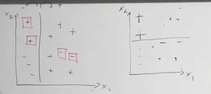
So after the first image, we have depth one DT, and we have some incorrect predictions. So, we increase the weight of these data points, and run again. Basically, we can determine, for classifier $G_{M}$ (every line we draw, every single DT, is a classifier), a weight $α_{m}$ which is proportional to how many right or wrong, so a better classifier, we want to give it more weight, and vic versa. For example, the equation used in AdaBoost is $1/2 l o g (\frac{1 - er r _{m}}{er r _{m}})$ .

So, the total classifier is some function $G (X) = \sum_{m} α_{m} G_{m}$ where each $G_{m}$ is trained on a re-weighted training set. Let’s examine in particular, AdaBoost

AdaBoost

Let’s see how to work with AdaBoost with Decision Trees, as this is the most common way to use AdaBoost.

https://www.youtube.com/watch?v=LsK-xG1cLYA&ab_channel=StatQuestwithJoshStarmer

In a Random Forest, each time you make a tree, you make a full-sized tree:

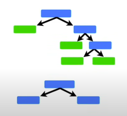
There is no determined max-depth.

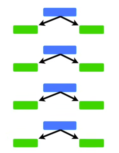
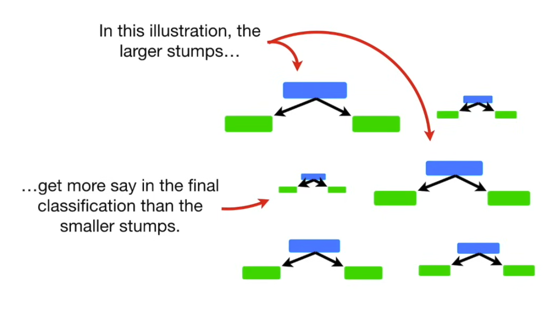
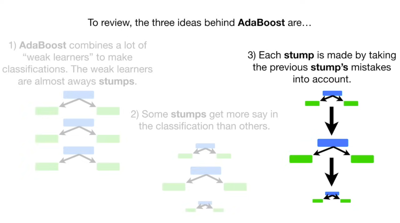
In a Random Forest made with AdaBoost each tree has depth 1 → called stumps → forest of stumps. Stumps are not great at making accurate classifications, and are technically weak learners. We know that in random forest, each trees vote has equal say in the final classification, whereas with AdaBoost, we assigned weights to the classifiers, so some of them are more important than others.

Lastly, in Random Forest, each DT is made independently of others. In contrast, with AdaBoost, order is important. The errors that the first stump makes, influence how the second stump is made, and so on and so forth.

Let’s see an example of how we can create a forest of stumps using AdaBoost. 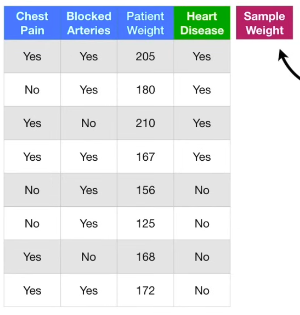The first thing we do, is to give each sample a weight that indicates how important it is to be correctly classified. In the beginning, all samples get the same weight, so for this, 1/8, meaning they are all equally important. So, we need to make the first stump. This is done by finding the variable: chest pain, blocked arteries, patient weight, that does the bets job of classifying the samples.

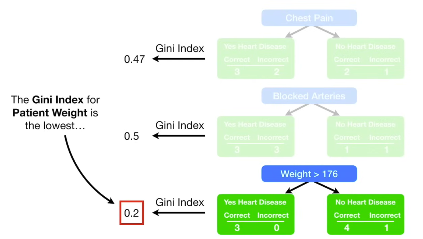
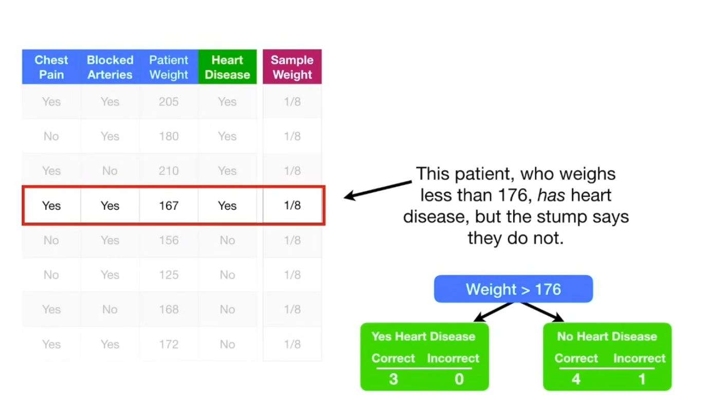
So, this is the first stump in the forest. Now, we need to determine how much say this stump will have in the final classification → determine by how well it classified the samples. So, in this case, total error is 1/8. We use the total error to determine the amount of say (influence) of the this stump in the final classification, using the formula $\frac{1}{2} l o g (\frac{1 - er r _{m}}{er r _{m}})$ , so for the above example, the weight is 0.97. Now, we update the sample weights: $new weight = sample weight \cdot e^{amount of say}$ , so for this example, would be $\frac{1}{8} \cdot e^{0.97} = 0.33$ which is an increase in weight. 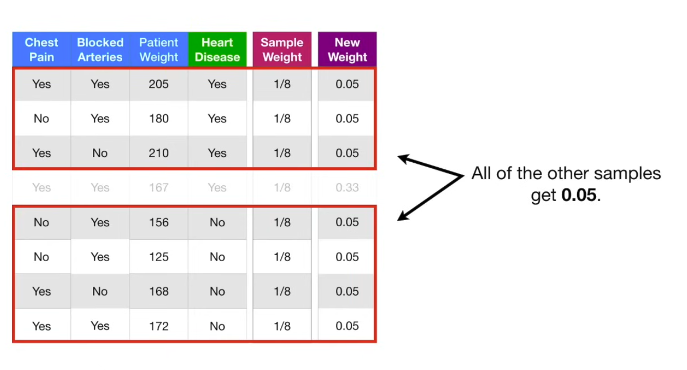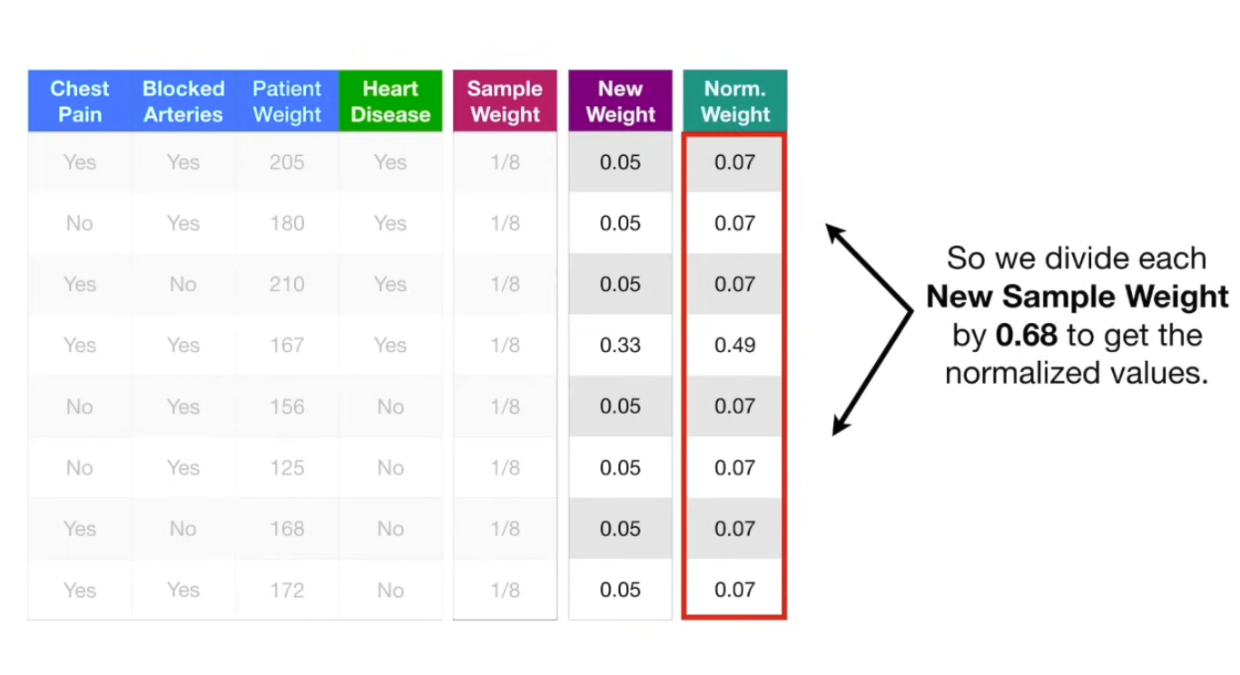Now, we decrease sample weights for the correctly classified ones: $new weight = sample weight \cdot e^{-amount of say}$ .

Then, we move those back into the sample weight column, and move onto creating the second stump.

💻 Allan Yin's Blog

Explorer