Chapter 3- Support Vector Machines

This chapter, we introduce the concept of SVM: Support vector machines. This area of machine learning excels in classification tasks. If we think of all our data in some high dimensional space, SVM seeks to find the hyperplane that separates the points of 2 different categories onto opposite sides of the hyperplane. This note will deviate from the course notes, in that, where math heavy is necessary, I will write and explain. But, for areas where it is redundant and easier to explain with words + diagrams, I will make that substitution. Please still review course slides in addition to this, thought once you have reviewed this, course slides should only be ~10 minutes of reading, and mostly review. The diagrams are sources from this video:

Support Vector Machines: All you need to know!

MachineLearningDeeplearningSVM
https://www.youtube.com/watch?v=ny1iZ5A8ilA&ab_channel=IntuitiveMachineLearning

---

Overview

SVM are a form of non-linear supervised machine learning models, where given some labeled training data, SVM will help help us to find optimal hyperplanes which categorize new examples. Let’s see an overview on how to find this optimal hyperplane. Consider the following sets of data:

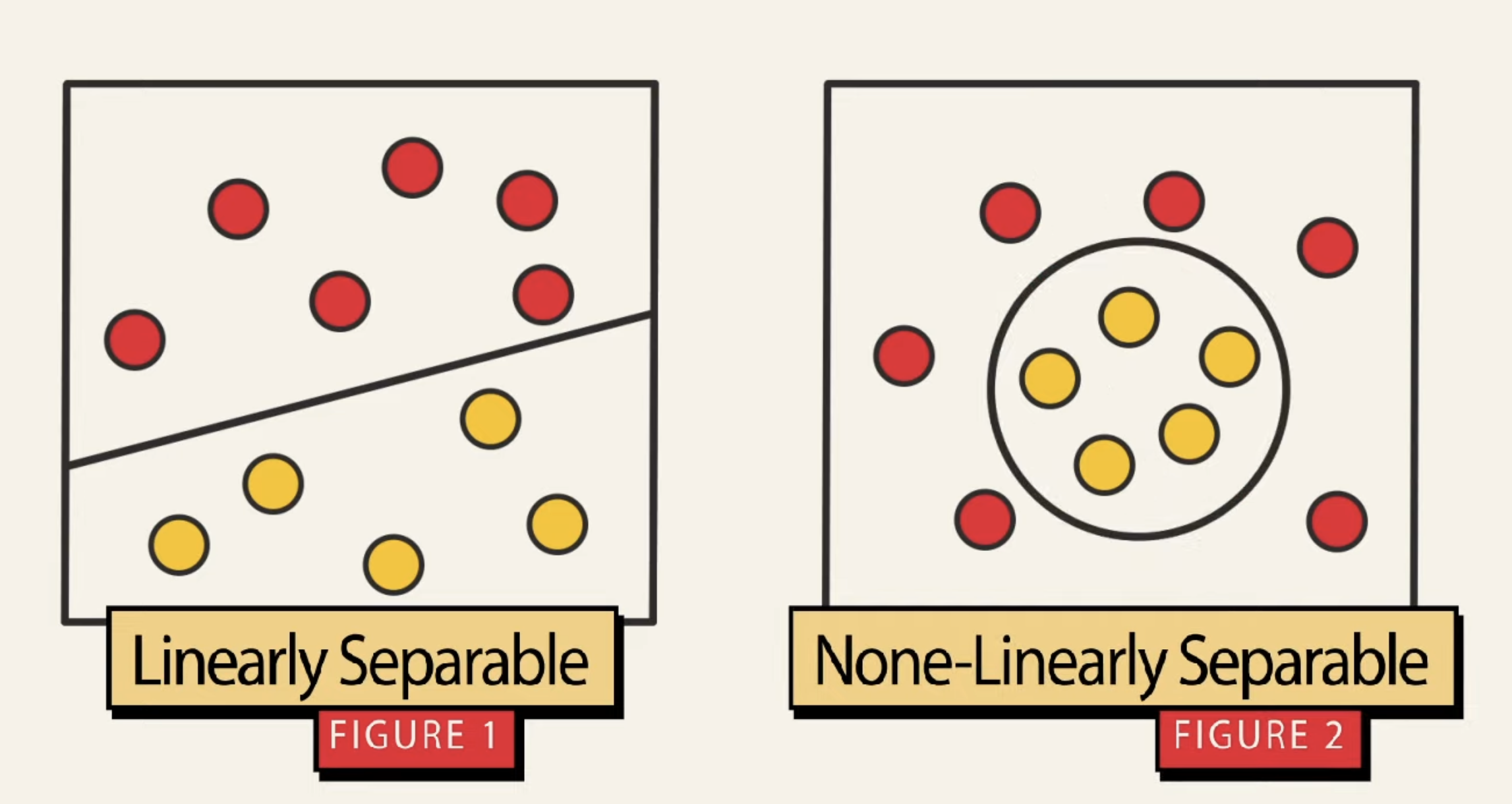
Let’s have a close look at figure 1. Amongst that data, there are multiple hyperplanes that can be drawn to separate the 2 classes of data. Which one is the best? SVM helps us choose the best hyperplane by maximizing the margin: the margin is the distance between the hyperplane and the nearest data point from either class. By maximizing this margin

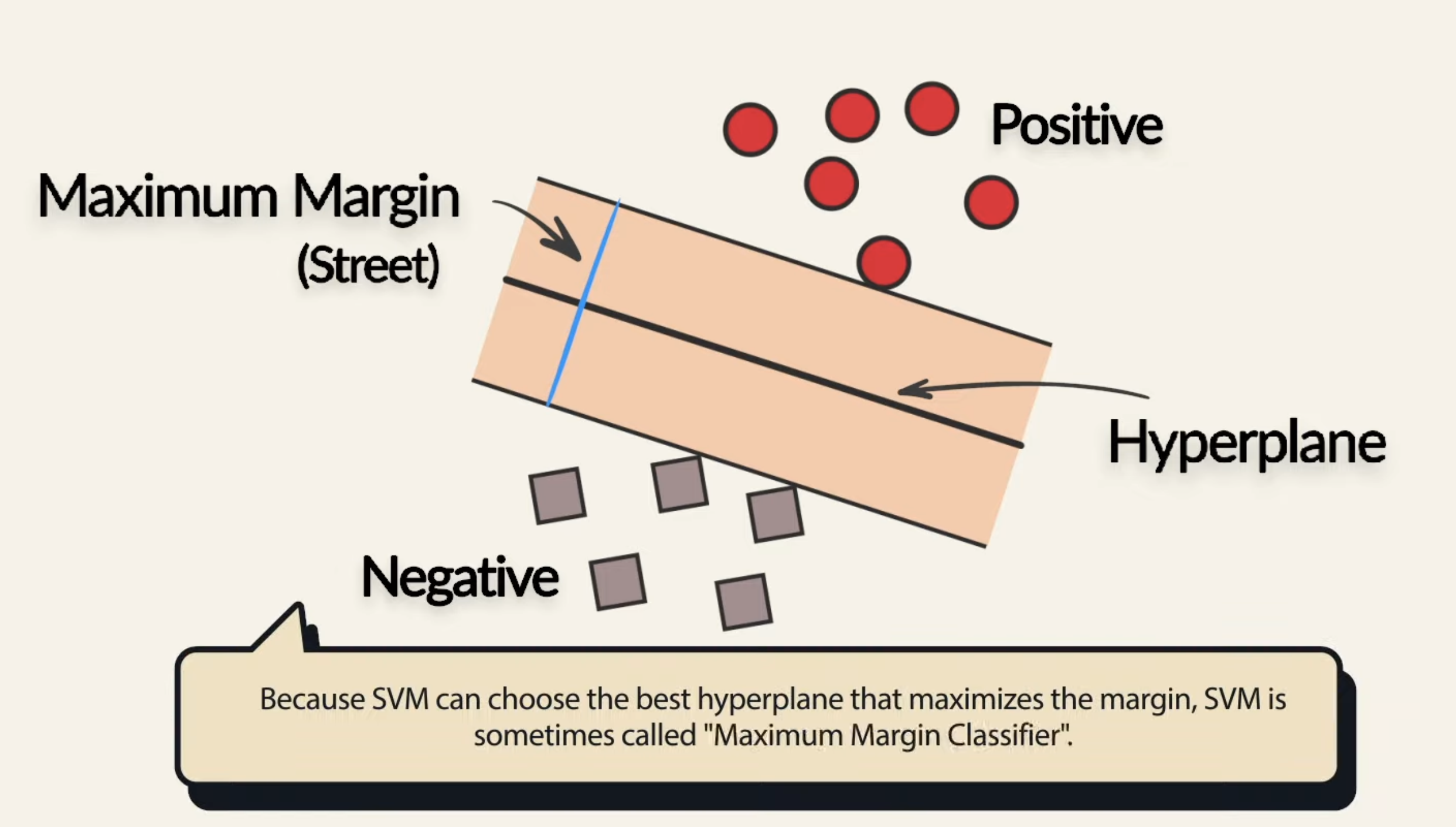
Now let’s introduce another concept: Support Vectors. These are the data points that lie closest to the hyperplane, and thus the most “difficult” to classify. Unlike other models such as regression or neural networks (where every data point influence the final optimization), for SVM, only the difficult points, the support vectors, have an impact on the final decision boundary. So, moving the support vectors alters the hyperplane, but moving data points that are not the support vectors, does nothing.

In essence, the concept of SVM is very similar to perceptron, where we are given a set of input data $X$ and in order to predict the corresponding labels $Y$, we multiply our data by a weight and add a bias: $WX+b=Y$. So, from this, you might wonder “this is just like a basic dense layer in a neural network, whats the difference then?”. However, there is a major difference, in that, SVM will optimize the weights in such a way, that only the support vectors determine the weights and decision boundary. Let’s go through a high-level look at the mathematics:

Mathematics Overview

Consider the following diagram:

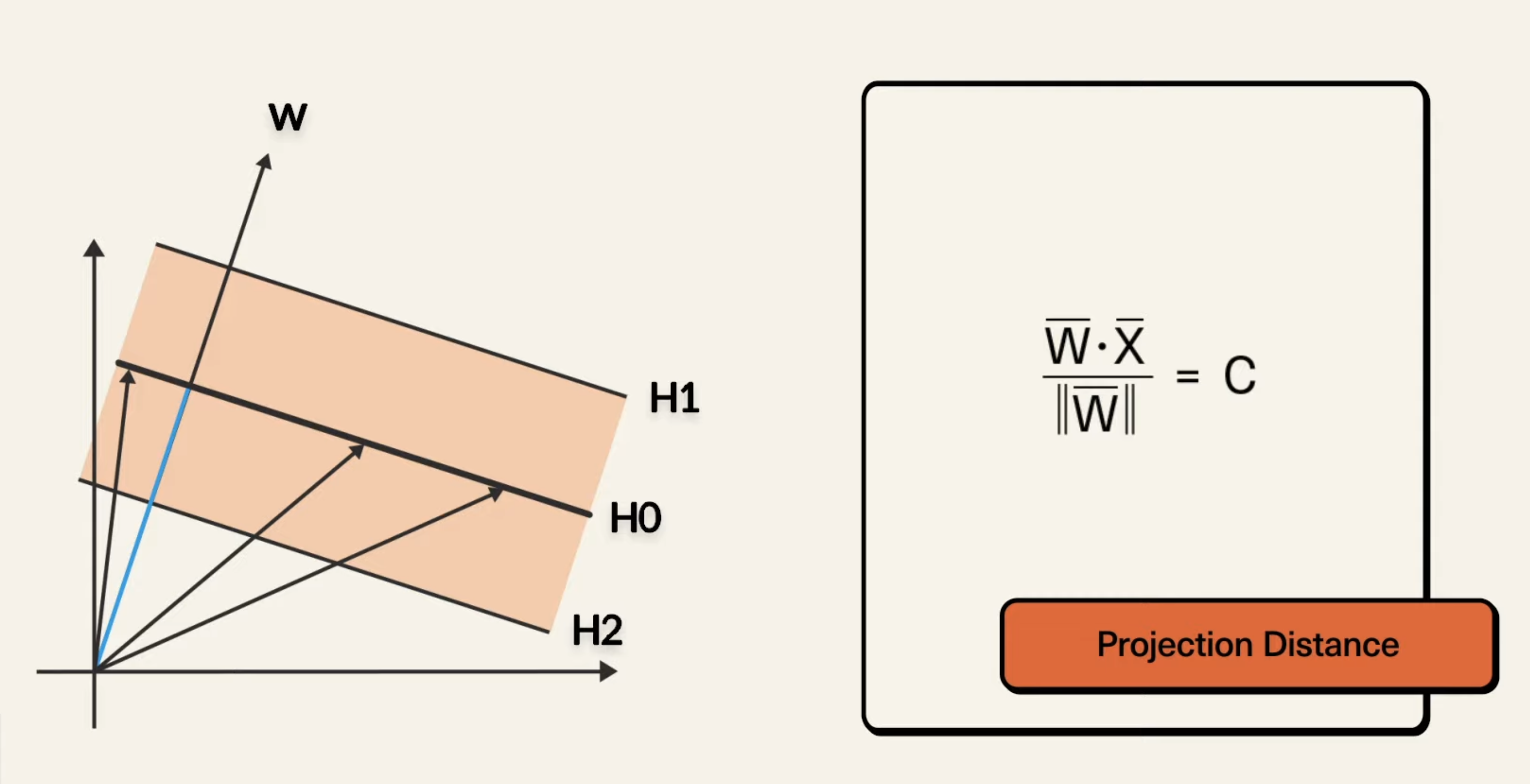
Then, multiplying both sides, we can obtain $\bar{W}\cdot \bar{X}=||\bar{W}||C$, and then we can substitute the right side with $-b$, so it becomes $\bar{W}\cdot \bar{X}=-b$, so, $\bar{W}\cdot \bar{X}+b=0$. This is the equation of the hyperplane $H_0$ in the above. This formula is for the 1D hyperplane (recall in an n-dimensional space, a hyperplane is an (n-1)-dimensional subspace). If we wanted to generalize the above hyperplane equation to 2D, we would have something like: $W_1{X}_1+W_2{X}_2+b=0$, and so on.

So, we have $\bar{W}\cdot \bar{X}+b=0$ are our hyperplane, which provides us with basic binary classification capabilities, where if we have $\bar{W}\cdot \bar{X}+b\ge 0$, then we predict the point as a “positive” sample, and “negative” if $\bar{W}\cdot \bar{X}+b<0$. Now, since we have equation for the hyperplane, we can easily find the equations for $H_1$ and $H_2$ above, being respectively $\bar{W}\cdot \bar{X}+b=k$ and $\bar{W}\cdot \bar{X}+b=-k$. To make things easier, we can scale the dataset so that we have $\bar{W}\cdot \bar{X}+b=1$ and $\bar{W}\cdot \bar{X}+b=-1$. To show a way to express the margin, we introduce 2 vectors:

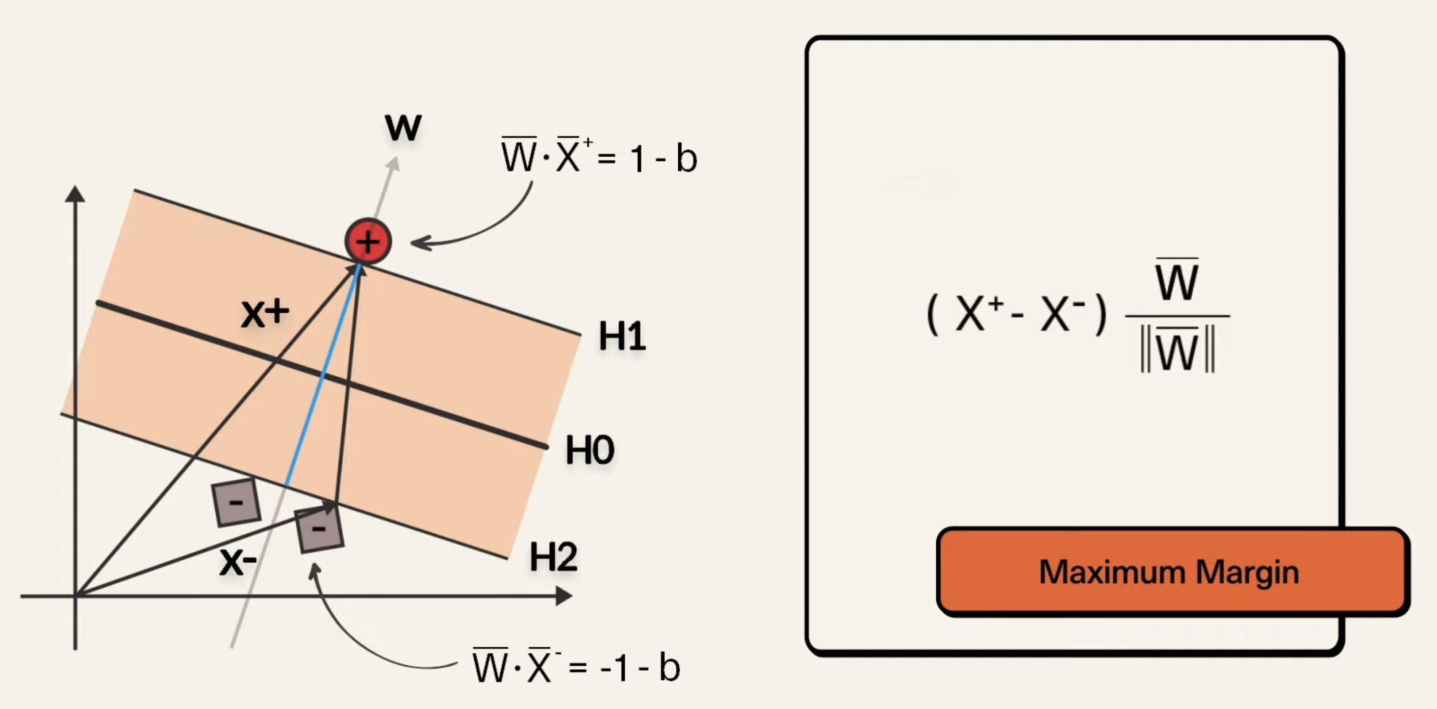
What the above shows is this:

• We have our vectors that point to a positive and negative point respectively
• Then, we take the difference of the 2 vectors (which is the black vector on the right of the blue line) and dot product it with unit vector perpendicular to $H_0$, and we can get an expression for the width of the margin. The equations for $H_1$ and $H_2$ follow the derivation above. So, in the above image, that expression can be simplified by multiplying the numerators, and then substituting the equations for $H_1,H_2$ in, which ultimately becomes: $\frac{2}{||\bar{W}||}$. This value is the simplified margin width, so, to maximize the width, we need to minimize the magnitude of $W$. For mathematical equivalence, it is the same to minimize $\frac{1}{2}||\bar{W}|{|}^2=\frac{1}{2}||\bar{W}||\cdot ||\bar{W}||$. But, we cannot keep increasing this width, we have a constraint (max something with constraint, …, CO lol). We have the constraint that no points will be inside of the margin, and so, we have:

  • For all positive points: $\bar{W}\cdot \bar{X}+b\ge 1$

  • For all negative points: $\bar{W}\cdot \bar{X}+b\le 1$

Now, the above can be simplified into one equation, and greatly resembles what we were doing in perceptron:

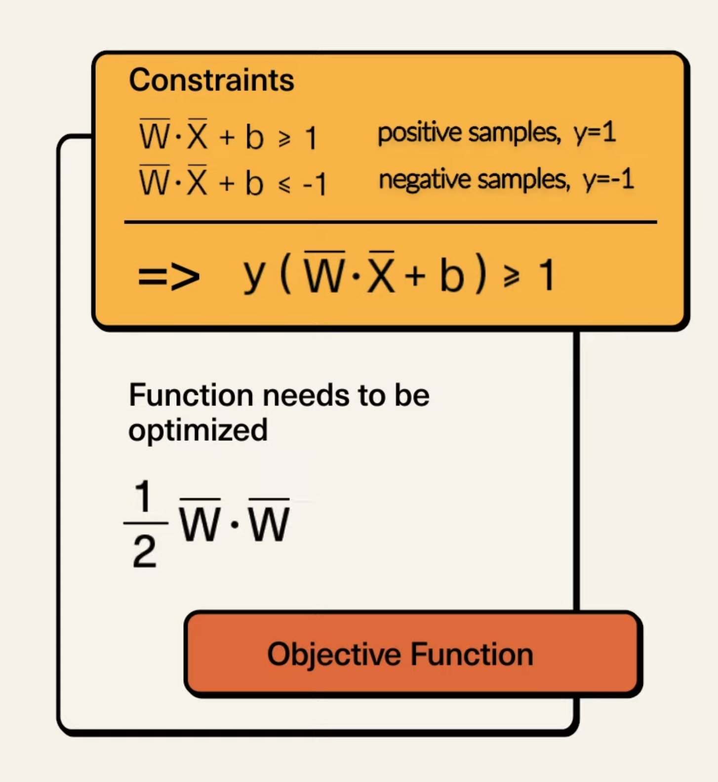
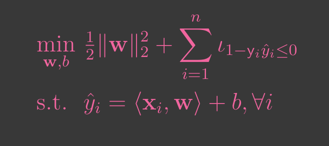
So, the above minimization problem of SVM is our Primal, which we can rewrite more clearly:

\begin{array}{ll}

Where:

• $\bar{W}$ is the weight vector

• $b$ is the bias term

• ${\bar{X}}_i$ is the i-th training sample

• $y_i$ is the class label of the i-th training sample (either +1 or -1).

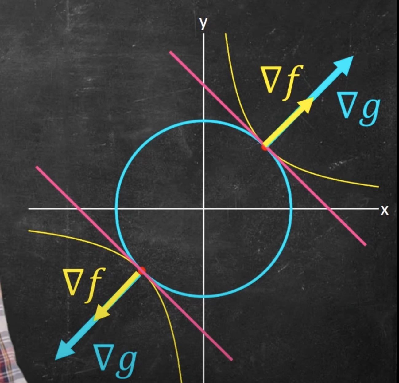
We solve this with Lagrange multipliers, and more specifically, Lagrangian Dual. So, we need to find the dual problem first, which we use Lagrange multipliers for. We introduce a Lagrangian multipliers ${\alpha }_i\ge 0$ for each constraint. This gives us the function: $L=\frac{1}{2}||\bar{W}||\cdot ||\bar{W}||-\sum {\alpha }_i[y_i(\bar{W}\cdot {\bar{X}}_i+b)-1]$. To find the dual, we take partial derivatives of $L(\bar{W},b,\alpha )$ with respect to $\bar{W}$ and $b$, and set them to 0. Why is this? Recall that when we looked at Lagrange multipliers, we saw:

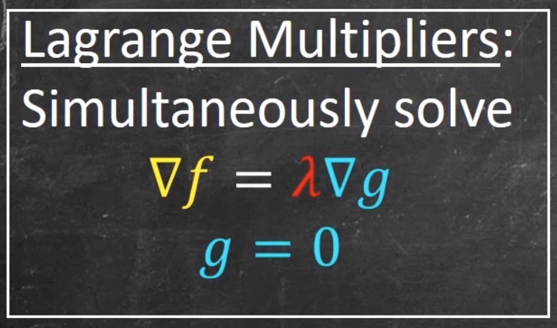
Where f is obj func and g is constraint

So, we take gradient (hence why are taking partial derivatives in the above). Taking the partial derivatives with respect to $\bar{W}$, we get:

$\frac{\partial L}{\partial \bar{W}}=\bar{W}-{\sum }_i{\alpha }_i{y}_i{\bar{X}}_i=0$

Same for $b$:

$\frac{\partial L}{\partial b}=-{\sum }_i{\alpha }_i{y}_i=0$

Substituting $\bar{W}$ back into the function $L$, we get the dual problem (this is in course notes, too, so no need to re-write later on):

\begin{array}{ll}

In hindsight, a lot of the dot products above weren’t written with <>__, just keep that in mind, same thing though

Now, we can easily multiply objective function to make this a min problem (as is in the course slides). The dual problem is often easier to solve and provides the same solution as the original optimization problem. Once you solve the dual problem, you’ll get the optimal values for the Lagrange multipliers ${\alpha }_i$. The support vectors are the data points for which ${\alpha }_i>0$. These are the points that lie on the margin. Then, we compute the hyperplane via weight normal vector $\bar{W}$. Also, with the above $\bar{W}$ derivation, we can re-write the equation of the hyperplane and alter the decision boundary rule:

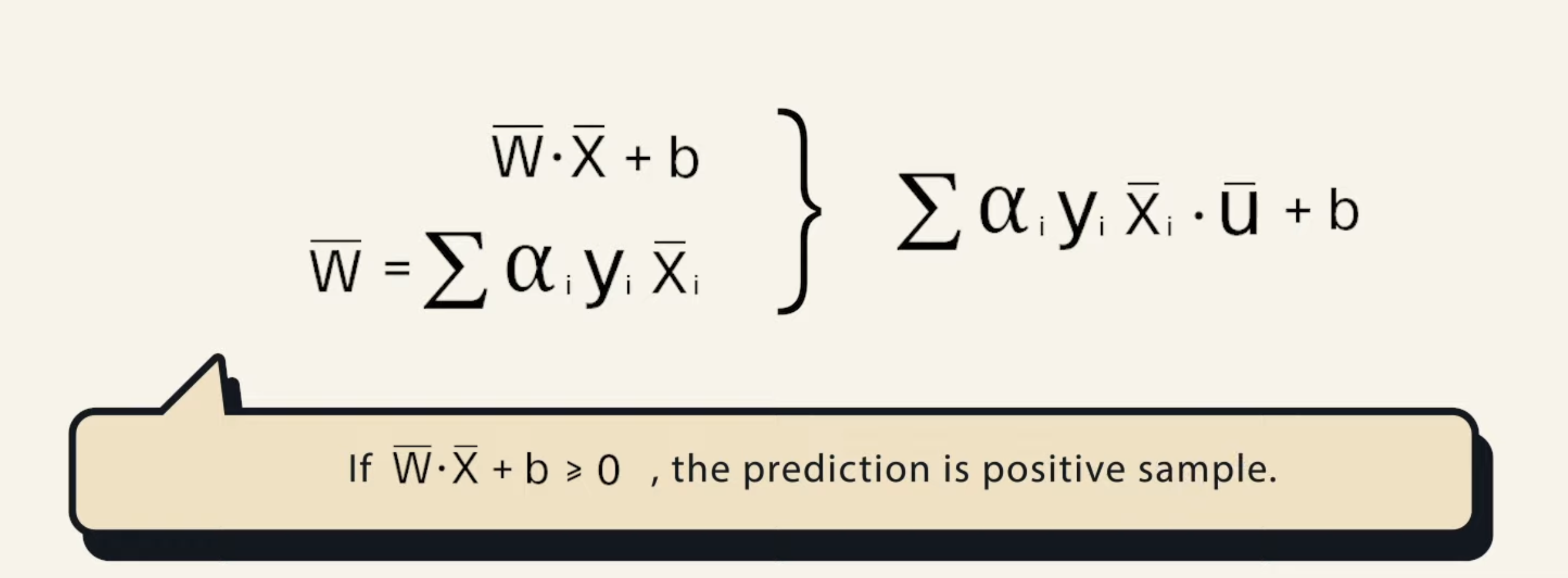
Then, to find bias, we take any support vector ${\bar{X}}_s,y_s$, and compute: $b=y_s-\bar{W}\cdot {\bar{X}}_s$, and for stability, we may often choose to take the average $b$ over all support vectors. Now that we have weight and bias, we have model for classification.

This has all been hard-margin SVM, and we are operating under the pretence that the data is linearly separable. In cases where the data is not linearly separable, we would use soft-margin SVM, which we will detail in the below. Next, we will look at another technique to combat data that is not linearly separable, but that we want to use SVM for classification, called kernel trick.

---

Soft-margin SVM

So, in the above hard-margin examples, we’ve operated under the assumption that the data points were linearly separable with not outliers. When if there is some noise and outliers in the dataset? For example, what if we had something like:

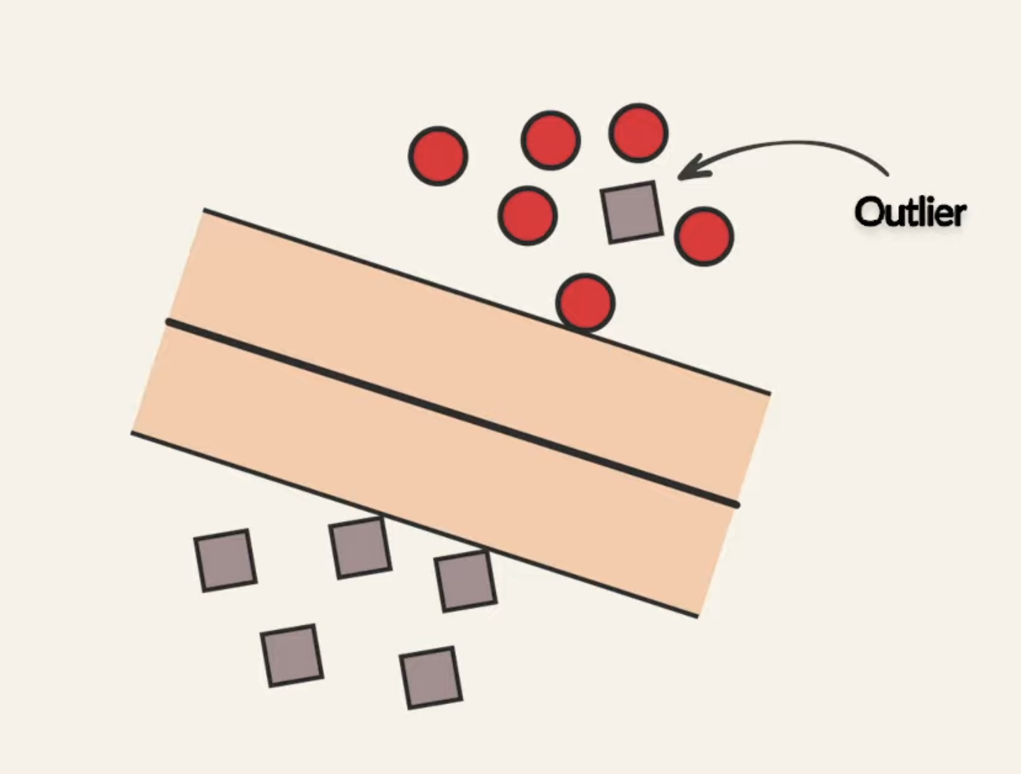
For something like this, hard-margin SVM would fail to find the optimization for the hyperplane. In hard-margin, in order for a data point to be classified as positive, we need it satisfy the condition: $Y_i(\bar{W}\cdot {\bar{X}}_i+b)\ge 1$. We now address this limitation with soft-margin SVM. First, let’s add a slack variable to the right hand side of that inequality, providing us with:

$Y_i(\bar{W}\cdot {\bar{X}}_i+b)\ge 1-{\zeta }_i\forall i=1,m,\zeta \ge 0$

Without slack variables, the SVM would be forced to find a hyperplane that perfectly separates the data, which may not exist. The slack variables allow for some miss-classification, and helps the model to find a balance between margin width and classification accuracy. The introduction of slack variables provides a way to control the trade-off between maximizing the margin and minimizing the classification error. This is done through the regularization parameter $C$ in the objective function → this is L1 Regularization, adding some kind of penalty for large values of $\zeta$. The regularized objective function becomes:

$\frac{1}{2}||\bar{W}||\cdot ||\bar{W}||+C{\sum }_{i=1}^m{\zeta }_i$

We note that $\zeta \ge 0$, so always positive, and the regularization parameter $C$ determines how important $\zeta$ should be, which intuitively represents how much we want to avoid misclassifying each training example.

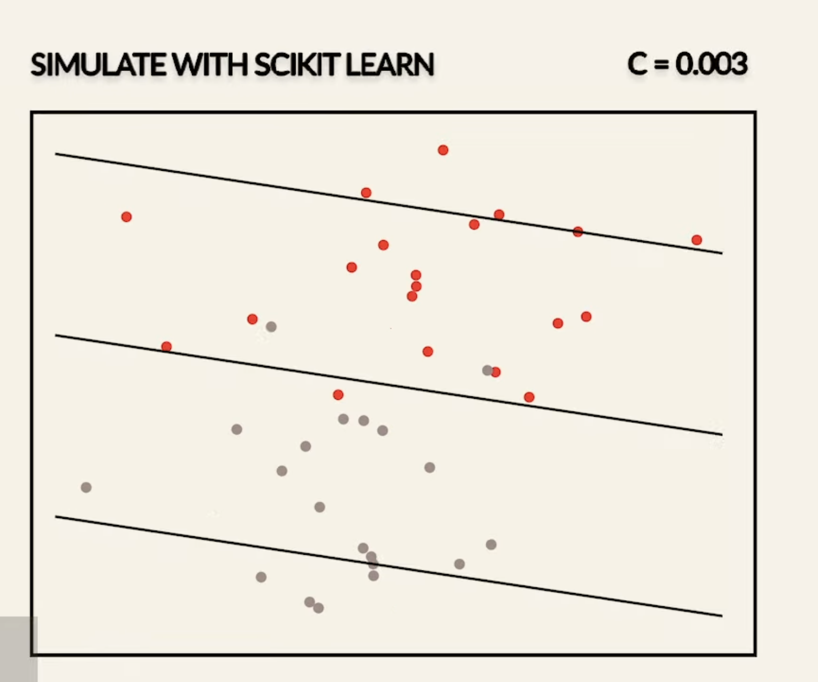
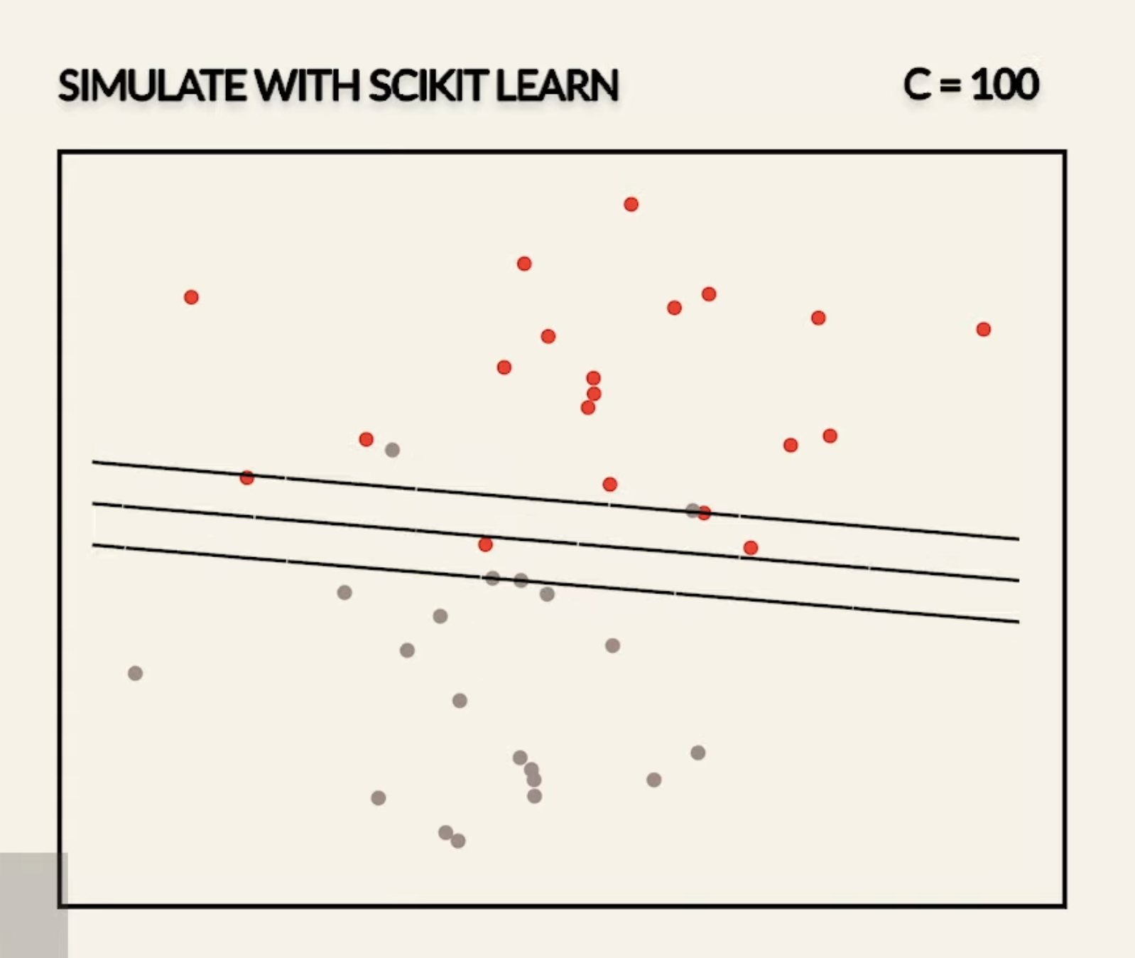
• Smaller $C$ emphasizes the importance of $\zeta$ and a larger $C$ diminishes the importance of $\zeta$
• In fact, if we set $C$ to be $+\infty$, we will get the same results as hard-margin SVM

So, smaller values of $C$ will result in wider margins at the cost of some misclassifications, and large values of $C$ will result in smaller margins, and less tolerant to outliers.

But this, is only for instances where there is some noise or outliers in the data, and otherwise, would have been separable. What if the non-linearly separable data is not caused by noise? What if the data are characteristically non linearly separable? For this, we can use the kernel trick

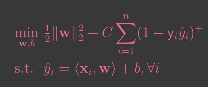
Now, in the lecture notes, instead of using this slack variable, we directly used hinge loss. Mathematically, the two approaches are equivalent in that they both aim to find the optimal hyperplane that maximizes the margin while allowing for some classification errors. The differences lie in how these errors are quantified and handled in the optimization problem. Hinge loss can be viewed as a streamlined or implicit way of incorporating the idea of slack variables. Rather than introducing ${\zeta }_i$ as separate variables, hinge loss directly measures and penalizes the violations of the margin constraints. In essence, we are defining the zeta to be the value of hinge loss, described below:

---

→ Hinge Loss

Hinge loss is a crucial concept in SVM, particularly in the context of classification problems. Hinge loss is used to measure the error of a classifier, specifically in the context of SVMs. It is designed to ensure that not only do we classify data points correctly, but we also classify them with a sufficient margin. The hinge loss function is defined as follows:

• For a single data point $(x_i,y_i)$, we get:

• $L(y_i,f(x_i))=max(0,1-y_i\cdot f(x_i))$ where $f$ is the model, or in longer terms: $f(x_i)=W\cdot X_i+b$

So, how do we understand Hinge Loss:

• Correct Classification with Margin: If a data point is correctly classified and lies outside the margin (i.e., $y_i\cdot f(x_i)\ge 1$), the hinge loss is zero. This indicates the classifier is not penalized for this data point and is correctly classified with sufficient margin

• Incorrect Classification with Margin: If a data point is either misclassified or within the margin (i.e. $y_i\cdot f(x_i)<1$), the hinge loss is positive. The amount of loss increases as the prediction deviates from the desired margin, penalizing the classifier for errors and margin violations.

The objective of training an SVM is to find the parameters $w$ and $b$ that minimize a combination of hinge loss and regularization term. This can be formulated as:

Hard-Margin SVM

Soft-Margin SVM

$\frac{1}{2}||W|{|}_2^2$ is the regularization term that helps in maximizing the margin by penalizing large weights.

---

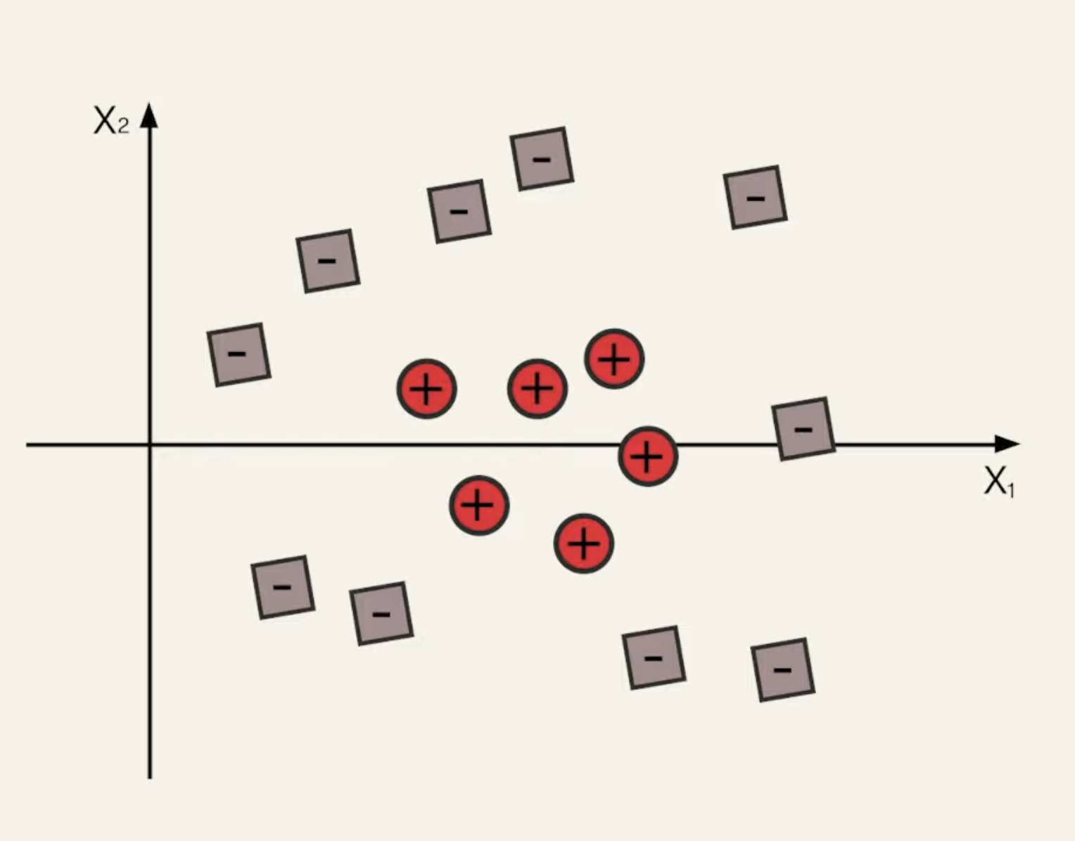
Let’s take a brief look at the Kernel trick, which we will deep dive into in the next chapter. This is especially important in situations when our dataset is non-linearly separable data. Consider something like:

If we lift this, then we can fit some higher-dimension hyperplane. Now, let’s revisit our Lagrange Equation:

$-{\sum }_i{\alpha }_i-\frac{1}{2}{\sum }_i{\sum }_j{\alpha }_i{\alpha }_j{y}_i{y}_j⟨{\bar{X}}_i{\bar{X}}_j⟩$

We can scale this to become our Kernel Function:

$-{\sum }_i{\alpha }_i-\frac{1}{2}{\sum }_i{\sum }_j{\alpha }_i{\alpha }_j{y}_i{y}_{j}k⟨{\bar{X}}_i{\bar{X}}_j⟩$

That is, the trick is to replace our dot product $⟨{\bar{X}}_i{\bar{X}}_j⟩$ with a newly defined kernel function $k⟨{\bar{X}}_i{\bar{X}}_j⟩$. This a small but powerful trick. For the above graph, we coan define $k=X_1^2+X_2^2$

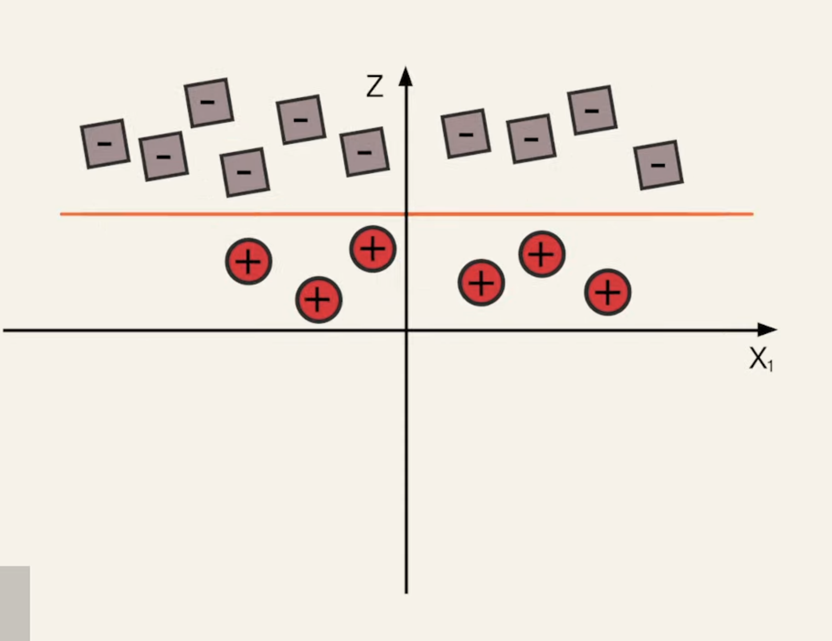
Notice that this is z dimension, so we’ve transformed our data into 3D space, and now, we can see a hyperplane.