Chapter 1- Perceptron

Perceptrons are the fundamental machine learning model, and many things, like Neural Networks and Transformers are built upon the concepts found in perceptrons. Its as simple as it gets. This is the introduction to machine learning, so we’ll go over everything.

The below is an amazing overview of dot-products and their role in linear transformations.

Dot products and duality | Chapter 9, Essence of linear algebra

Why the formula for dot products matches their geometric intuition.
https://www.youtube.com/watch?v=LyGKycYT2v0&ab_channel=3Blue1Brown

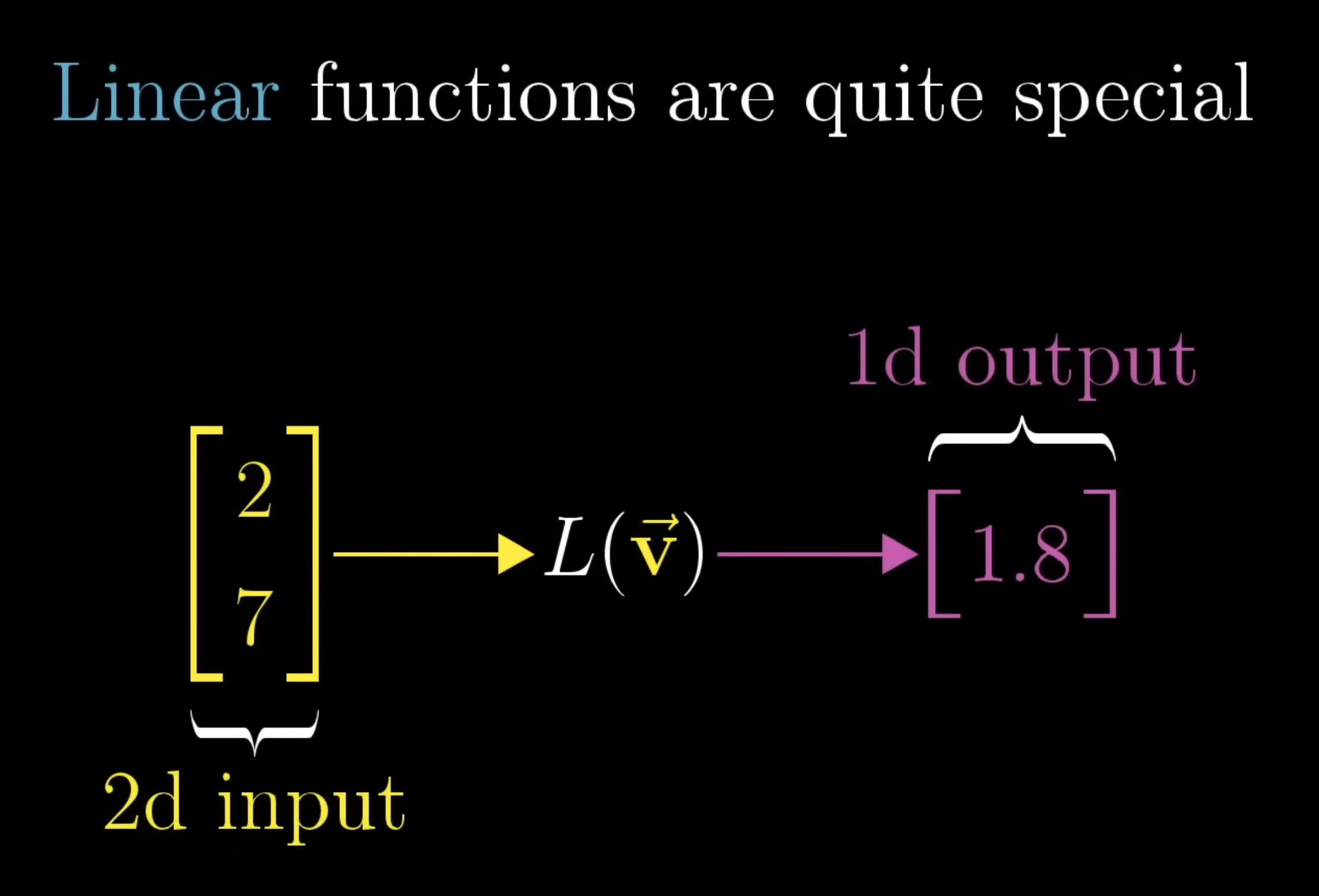
Something important to mention is the concept of linear transformations from higher dimensions into one-dimension, as this is essentially what we are doing with a dot-product between vectors. In the domain of 2D vectors, they’ll encompase something like:

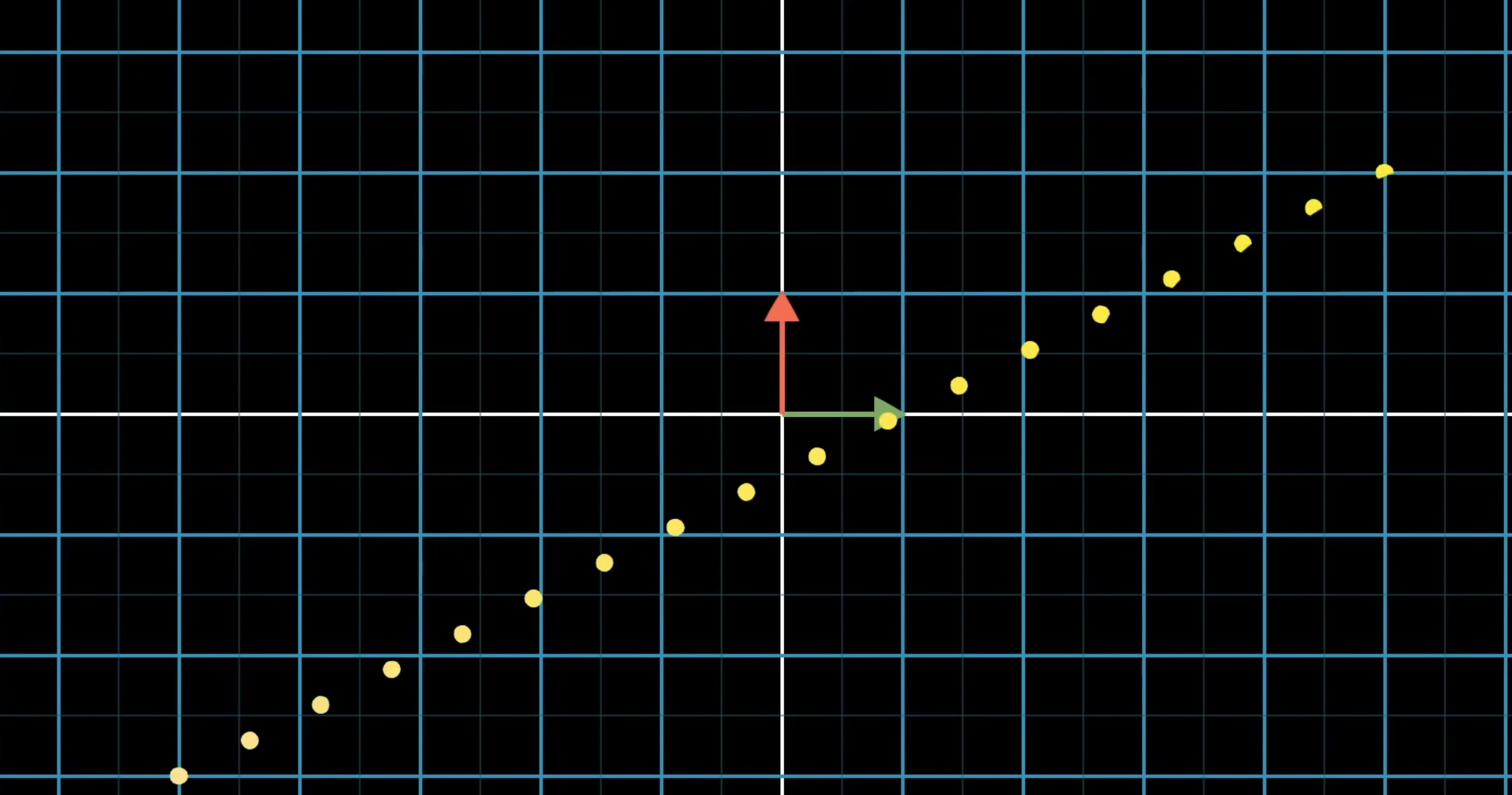
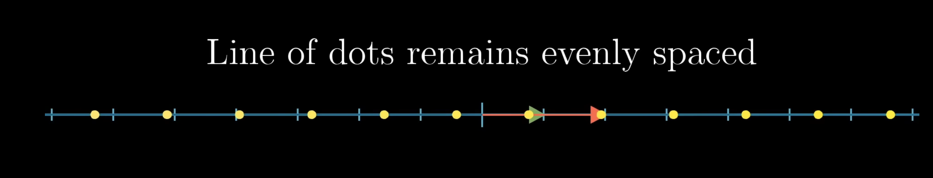
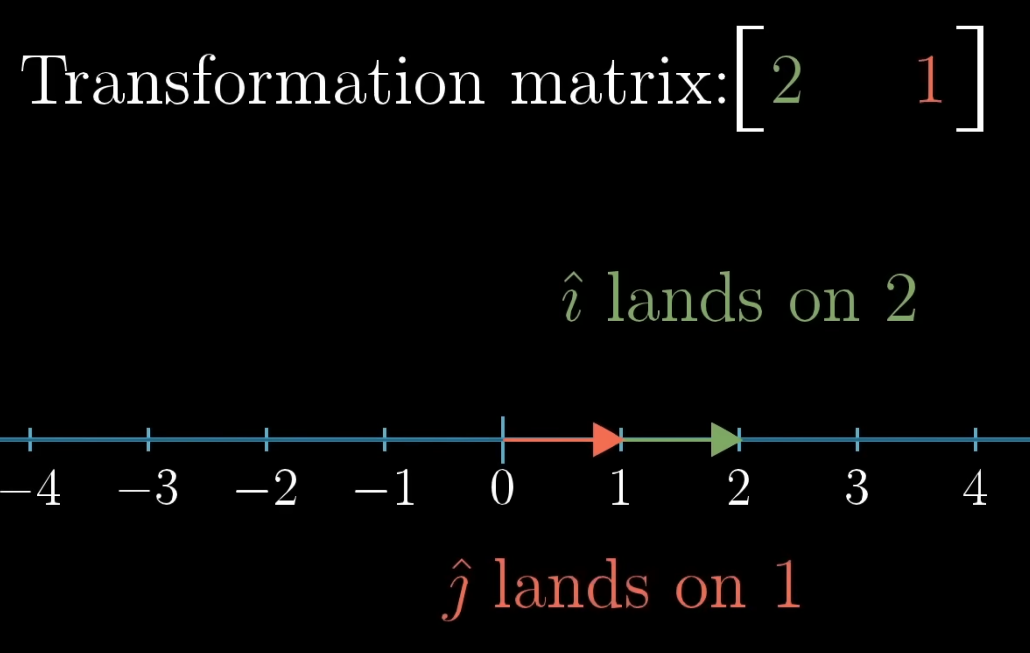
Let’s ignore the formal definitions of linear functions, as those aren’t much help in understanding the geometric meaning of this. If we were to take some line of evenly spaced dots in 2D and applied some linear transformation to it, a linear transformation about keep these dots evenly spaced in the output space (the number line):

A linear transformation is determined by where it takes $\hat{i}=[1,0]$ and $\hat{j}=[0,1]$ in the number line. In a the context of a linear transformation into 1D, each of them land on some specific number on the number line.

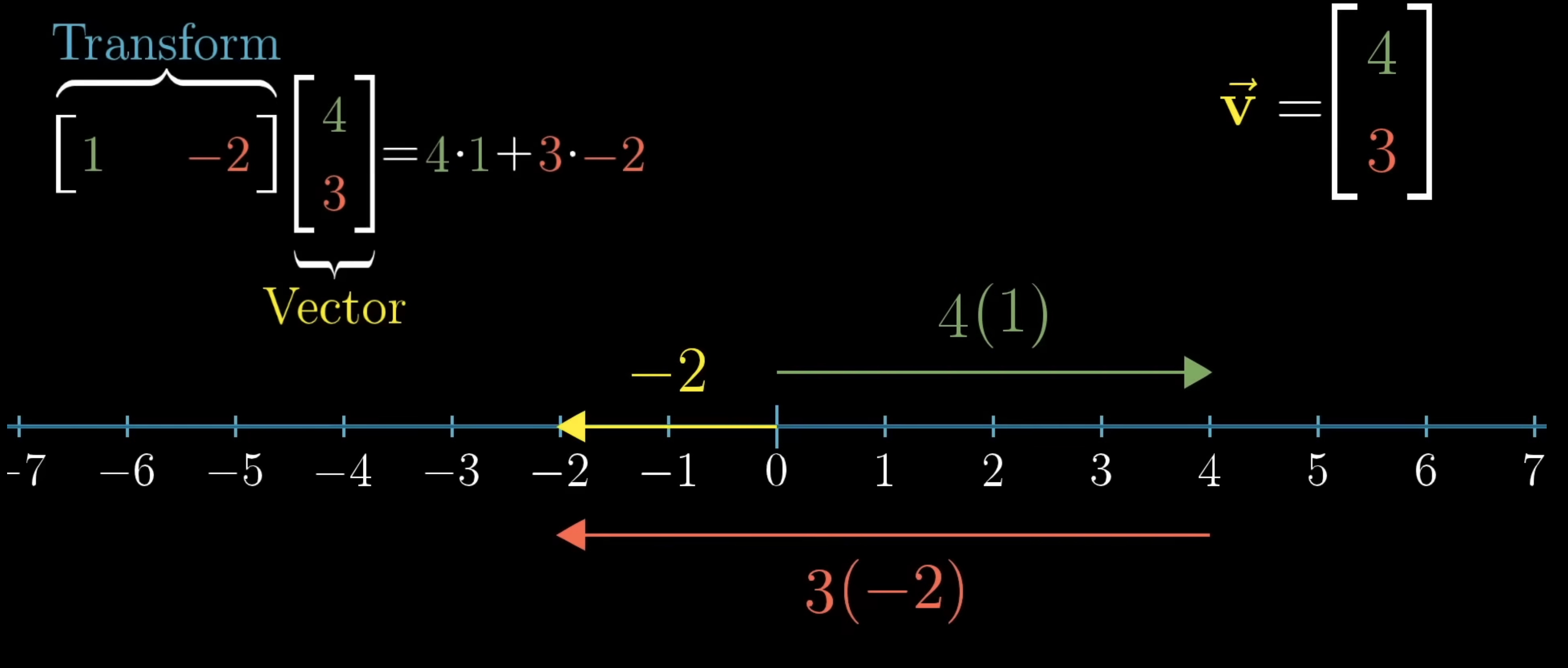
So, what does it mean to apply one of these transformations to a vector? So say we had something like: $[4,3]$. We break this into its $\hat{i}$ and $\hat{j}$ components → so we’re just 4 and 3 times the places where $\hat{i}$ and $\hat{j}$ land. Notice that if we do this, this is just the normal dot product that we are familiar with.

So, this shows us that linear transformations into the one-dimensional line is the same as performing dot product. Let’s explain this more. We have $\hat{i}$ and $\hat{j}$ which are our basis vectors. Now, whatever linear transformation into the 1D we use, each of the basis vectors will be mapped to some point. Take the above picture as an example:

• We have the basis vectors $\hat{i}$ and $\hat{j}$ to $[2,1]$. So, what would this linear transformation map the vector $[4,3]$ to? Well, we could break it into its basis component vectors.

• When we do this operation purely numerically, it is performing the matrix multiplication between the 2, as seen above → same as dot product

• So this shows us any linear transformation from a higher dimension into the 1D number line, can be modled with one $1$ x $n$ matrix matrix multiplied against the vector in the higher dimension

This suggests something unseen, some kind of connection between linear transformations that take vectors to numbers, and vectors themselves. The lesson here, is anytime you have one of these linear transformations whose output space is the number line, no matter how it was defined, there is going to be some unique vector $v$ corresponding to that transformation, in the sense that applying that transformation is the same as taking a dot-product with that vector.

In summary, one the surface, the dot product is a very useful geometric tool for understanding projections and for testing whether vectors tend to point in the same direction, and this is probably the most important thing to remember. But at a deeper level, doting 2 vectors together is a way to translate one of them into the world of translations.

==→ When to use them?==

Perceptrons are basic machine learning models that are applicable when we have a dataset that is linearly separable → hence, it is most applicable for binary classification tasks. Before we go into detail on what they do, I’ll quickly describe what kind of data we are dealing with, how we quantify it, and how they are consumed by these models.

==⇒ Dataset==

Consider the following visual:

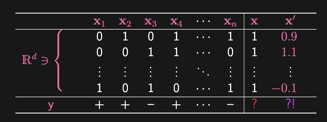
• This is an demonstration of a dataset. We have $n$ columns, meaning we have $n$ samples in the dataset. There are $d$ rows, which means we have $d$ features for each sample in the dataset. We need the data to be representable in numerical form, hence why use techniques like one-hot encoding when dealing with bags of words situation.
• What about the 2 right-most columns? Those represent our test data. How well our model performs on training data is relatively irrelevant, as over a large (or small) number of epochs, any sufficiently well-designed model will fit (and perhaps quickly overfit) to the training data. Our real interest is in the performance of the model on validation and test datasets. You’ll see, while the training and validation ($x$ with no subscript) data may contain binary data, its possible for test data to not conform to this expectation.
• What about the last row? The $y$ represents the label. Perceptrons are a form of supervised learning, where we already know what the correct classification is for the data point. So in this case, we have 2 classes: +1 and -1, and we already have classification for each of our $n$ samples.

  • Now, in binary classification, we don’t always assign -1 and +1 as labels, but they work well in these certain examples for basic loss function, which you will see later.

Let’s take a quick example of this binary classification problem, in one of the oldest common applications: spam filtering. Again, consider the following dataset:

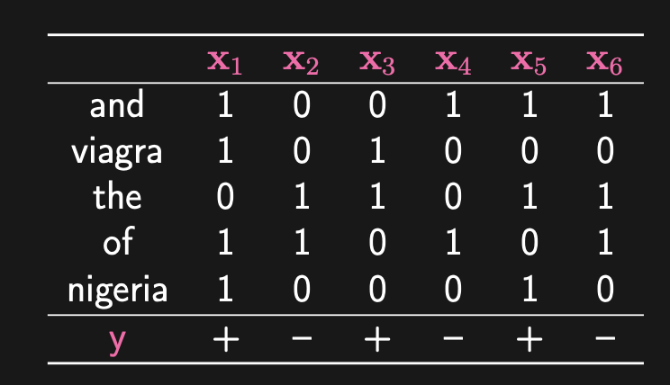
Same data spread as the above. Let’s also introduce some more formal mathematical notation to be used when describing this dataset:

• Training Set: $X=[x_1,...,x_n]\in {\mathbb{R}}^{d\times n}$, and $y=[y_1,...,y_n]\in \{\pm 1{\}}^n$ → remember, $y$ is label so it must be in this set

• This encoding technique is called Bag-of-words → used a lot in Natural Language Processing

You know that when training neural networks, the common approach is train via min-batches/batches. The perceptron model is based via online learning, so instead of computing some learning process based on a batch of data, we are doing so for each individual data point. Now, to jump into Perceptron models, we need a refresher on affine linear transformations/functions:

==⇒ Linear Threshold Function==

Consider the formal definition for a linear function (mathematical definition is of form $mx$, where no constant):

$\forall \alpha ,\beta \in \mathbb{R},\forall x,z\in {\mathbb{R}}^d\to f(\alpha x+\beta z)=\alpha f(x)+\beta f(z)$

And of course, we can have an arbitrary number of $\alpha$ and $\beta$, so it is better to represent this in vector notation, as below. Also, remember, the reason the input into the above function is $\alpha x+\beta z$ (which is any representable $d$-dimension vector) is because linear functions can take on vector inputs (just a function with $\ge 2$ parameters. Doesn’t matter how many, as long as the function only performs linear operations on those parameters, it is a linear function.

$\exists w\in {\mathbb{R}}^d\text{ such that }f(x)=⟨x,w⟩$

So by the above definition, we know the dot product formulation above is also a linear function. Knowing this, we can define an affine function

⇒ Affine Function

This concept is closely tied to linear functions. Affine functions are a extension of linear functions, where they add some constant to the end to make the line not pass through the origin. In the above, you can see that a linear function will always pass through the origin, as it has a constant bias of 0. Affine functions extend this to allow for this constant to be non-zero. Hence, we get the formal definition:

$\exists w\in {\mathbb{R}}^d,b\in \mathbb{R}\text{ such that }f(x)=⟨x,w⟩+b$

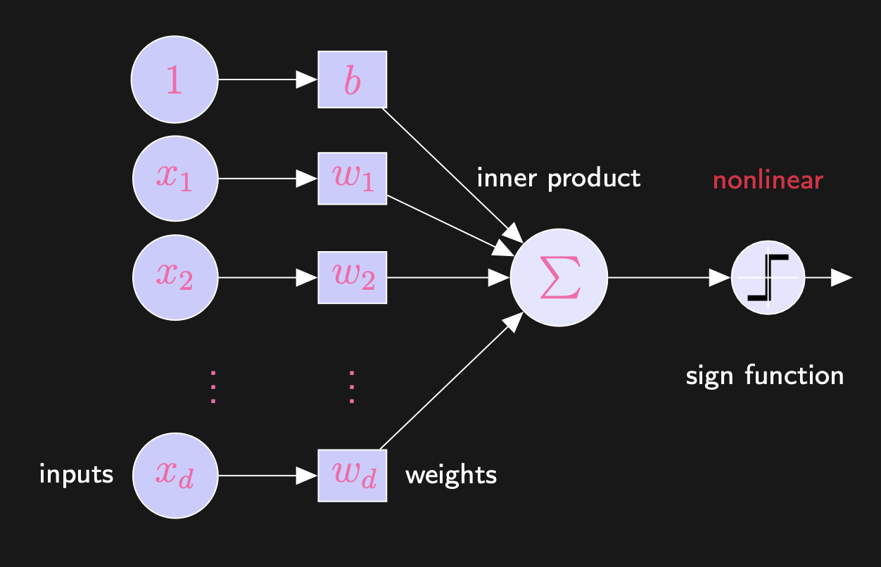
Before we can get to the final function for perceptron, here is the activation function for this:

⇒ Thresholding (Activation Function)

$f(x)=\{\begin{array}{ll}1& \text{if }t>0\\ -1& \text{if }t<0\\ ?& \text{if }t=0\end{array}$

We leave it as ? for $t=0$ since its really up to us to decide whether is something for that is considered $+1$ or $-1$. So, now that we have an activtion function, really, a perceptron sort of acts like a single neuron in a neural network:

$\hat{y}=\text{sign}(⟨x,w⟩+b)=\{\begin{array}{ll}1& \text{if }t>0\\ -1& \text{if }t<0\\ ?& \text{if }t=0\end{array}$

Note: In this class, we like to denote “hat” variables as our predictions.

Let’s see an example of the line that perceptron may draw in a binary classification task:

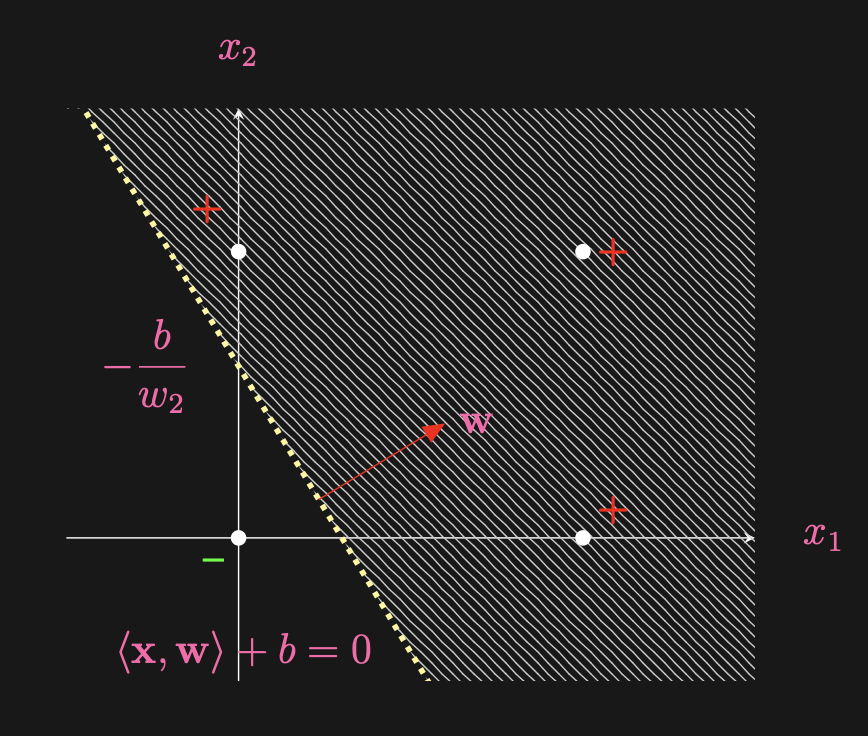
So, why is that for points above the line in the above diagram, we would have $⟨x,w⟩+b>0$? This is because what we mean by dot product (as mentioned above). While the anove

The graph should be fairly self-explanatory. The right diagram boils down the architecture of the perceptron (again, just a single neuron really). But for any classification task, there are many curves that are able to address the problem. Observe the following:

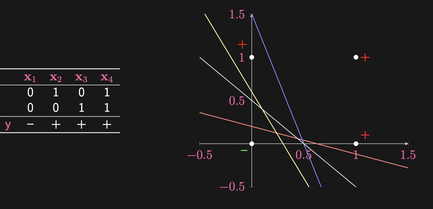
We’ll see later on how the algorithm decides on which line is best. Below is the pseudocode for the algorithm as well as a link to a colab page with the code so you can see source code:

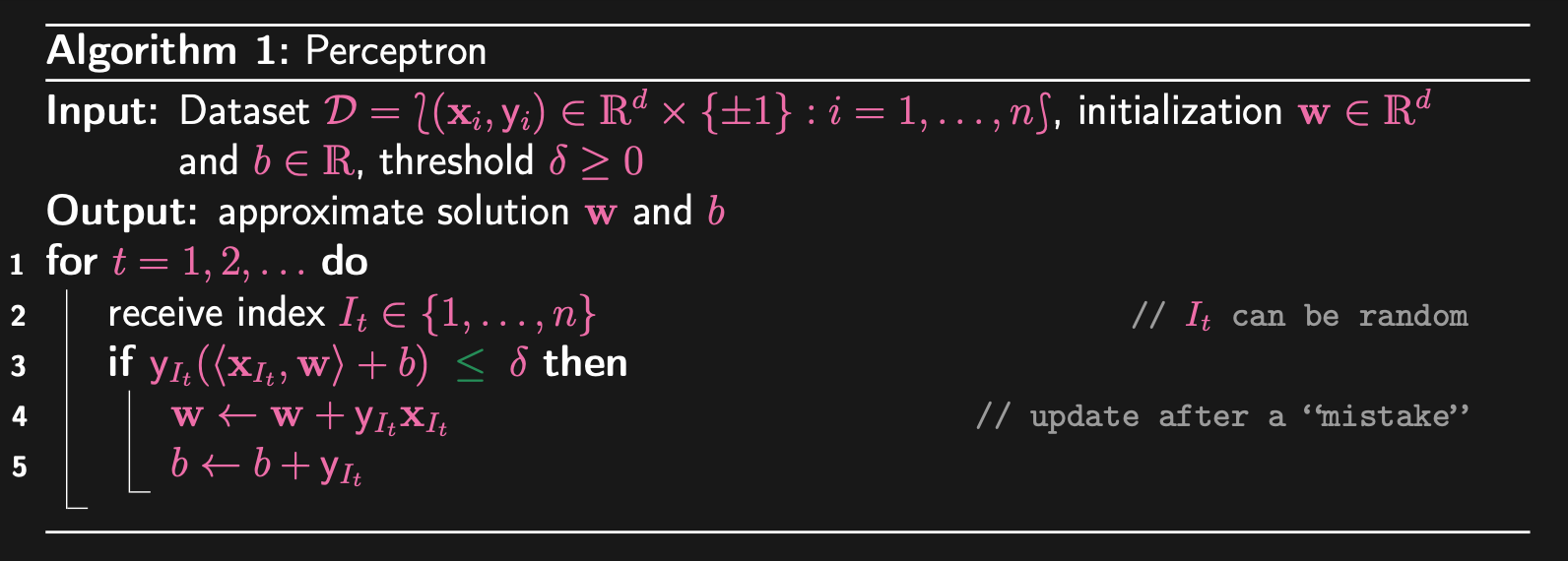
What is this doing? Let’s analyze this line by line:

• First, our dataset consists of our datapoints
• Every epoch, we are picking some datapoint (this is the receive index $I_t \in \{1,...,n\}$) and its label
• For this data point, we input it into the perceptron function from above. So, we are multiplying our weight $w$ by our data point $x_{I_t}$, adding the bias term, and the finally multiplying the value by $y_{I_t}$, which is the label.
  • We usually set $\delta =0$, as this is a good starting point (especially given the labels we have used in this binary classification problem), but it is definitely subjective to the problem at hand. This if statement is the fundamental loss function for this.
  • In the learning process (if we enter the if statement), we adjust our model weight ($w$) and and also adjust our bias
    • In this example, adjust model weight by subtracting $x_{I_t}$ from $w$ or adding it
    • For $b$, we are either incrementing it by 1 or decrementing it by 1
  • It is important to understand the geometric representation of multiplying the data point by the weight vector $w$.
    • The mathematical reasoning behind the dot product ==$⟨x_t,w⟩$ is finding the distance between the hyper plane performing the binary classification from the data point in the space of our data==
      • In fact, the vector $w$ is the normal of the hyperplane, and dot product as you already know, is extracting the component vector of our data point that lies in the direction of the vector $w$. Now, since we often initialize $w$ with 0, we need to add a bias term $b$ to allow the hyperplane to not be fixed at the origin.
    • This core geometric understanding is exactly how the perceptron model works — finding the distance to the hyperplane, and depending on whether this data point is lying in the correct half-space or not. If it is not (mis-classified), the perceptron model will shift the hyperplane minimally to accommodate for this missed point (at risk of thereby moving hyperplane over previously correctly classified data points).

The below is simulation of running perceptron to classify a list of points.

https://vinizinho.net/projects/perceptron-viz/

Interesting to note, we absolutely need the ==$\le \delta$. Why? Consider this:==

• We use only ==$<$, and $w=0$ vector, and $b=0$, then, if $\delta =0$ as well what happens? … nothing! So, we will be stuck here, no matter what data point we choose. This halts the learning and renders the model to be stuck in an infinite training loop, learning nothing.==

The danger of online learning is that we are updating model weights for every data point we train on. This can lead to the model “forgetting” past data, and performing wrong predictions on already seen data → though, this is sometimes necessary for the model to generalize.

• We can add a step size to the loss function to avoid jumping over local minimum

---

→ Monday May 13th 2024

This lecture, we finished off covering the Perceptron Model. In particular, we address the issue of convergence of the model. That is, given a dataset that there exists some hyperplane to perform binary classification, will the perceptron model, regardless of the scale of the data, be able to find this plane? The answer is yes, and we derive an upper bound on the number of “mistakes” (a.k.a number of times the model needs to learn) in order for our model to have 100% accuracy on the training set.

==Important note to self: While this is okay for very very simple functions such as Perceptron, anything that is more complex, we do not want this loss to be 0 → directly leads to overfitting and poor generalization power of the model. In order to maintain good generalization performance, we need to not 100% predict the training data. We’ll see this later on for sure.==

For convenience, moving forward, we will make a quick notation change. In particular, we can simply append the bias term to the end of the vector $w$, and append a 1 to the end of our data point vector, to avoid always writing that $+b$ term, and simply express this as a dot-product:

$⟨x,w⟩+b=⟨\left(\genfrac{}{}{0ex}{}{x}{1}\right),\left(\genfrac{}{}{0ex}{}{w}{b}\right)⟩$

==In the above, we define the first vector as $x$ and the second one as $z$==. In addition, we can move the multiplication of the label into the above:

$y[⟨x,w⟩+b]=⟨y(\genfrac{}{}{0ex}{}{x}{1}),(\genfrac{}{}{0ex}{}{w}{b})⟩$

Likewise, for the above, we can make the first vector ==$a$ and the second one stays $z$.== In this, we can boil this into a much simpler format:

$\text{find z}\in {\mathbb{R}}^p\text{ such that }{A}^{T}z>0,\text{ where }A=[a_1,a_2,...,a_n]\in {\mathbb{R}}^{pxn}$

The above is essentially, what the entire perceptron model boils down to → we are looking for some weight w, such that upon multiplying it across every data point, and summing those vectors, will result in a $n\text{ x }1$ vector, where the value of the result being $>0$ means that data point ($i$th row of the n rows) has been correctly classified.

If we format the perceptron model as the search for such a vector, we can now see a very strong relationship between. In that we are looking for a set of vectors that satisfies that above, we are looking for a cone of vectors. Since we are looking for all vectors $z$, we are basically asking for non-trivial linear combinations of the vectors $a_1,a_2,...$ that are greater than zero. This matches the definition of a cone:

A cone, in other words, it is the set of all vectors that can be formed by taking non-negative linear combinations of the given vectors.

---

Perceptron Convergence Theorem

→ Statement of the Theorem

Provided that there exists a strictly separating hyperplane, the Perceptron algorithm will iterate and converge to some weight $w$. If each training data point is selected infinitely often (which means the algorithm is choosing new random unseen data point), then for all $i$, we have $⟨y_i{x}_i,w⟩>\delta$. What about the special case, when we have set $\delta =0$ and initialized our model weight to be $w=0$. Then, perceptron converges after at most ${\frac{R}{\gamma }}^2$ mistakes, where:

$R:=ma{x}_i||x|{|}_2$

$\gamma :=ma{x}_{||w|{|}_2\le 1}mi{n}_i⟨y_i{x}_i,w⟩$

What is each of these representing? $R$ is the radius of the data set, that is, the maximum Euclidean distance of any feature vector $x_i$ from the origin in the $p$-dimensional feature space. We are looking for the maximum. Imagine if all our data was plotted on cartesian system ion 2D, then this would the point in our dataset farthest away from the origin.

What about gamma? Gamma represents margin, which refers to the separation or distance between the decision boundary (hyperplane) and the closest data point to the boundary. It quantifies how well-separated the classes are in the feature space. Let’s break down the formula above:

• $max(\Vert w\Vert 2\le 1):$ This is used to impose a constraint on the Euclidean norm of the weight vector $w$. This ensures that $||w|{|}_2$ is limited to values $\le 1$. So, it bounds the weight vector to a unit sphere/circle, etc.
• $mi{n}_i⟨y_i{x}_i,w⟩$: This part calculates the minimum signed distance between the data points $x_i$ and the hyperplane defined by $w$. This considers all data points, and ensures that $\gamma$ represents the smallest separation margin across all data points. This approach ensures that the margin calculation is invariant to the scale of the weight vector and focuses on the relative position of the data points with respect to the decision boundary.

Linear Separability: $\exists w\text{ s.t}⟨x_i,w⟩\ge s\ge 0$, where $s$ is some positive value

Now that we have defined these, we look to ==prove the convergence theorem.==