Chapter 6 - Convolutional Neural Networks

For this, we’ll jot down the most important mathematical notations, but for information on the how they work, what convolutions are, etc, please refer to the Deep Learning Folder.

Overview

Convolutional neural networks are the most tried and tested method in the field of image segmentation, recognition, and classification.

• When the input comes in, each convolutional layer is extracting features, and the output is feature maps. The number of feature maps is equal to the number of filters we have for that layer.
• The idea is, these feature maps become smaller and smaller, especially as we reduce resolution with max pooling
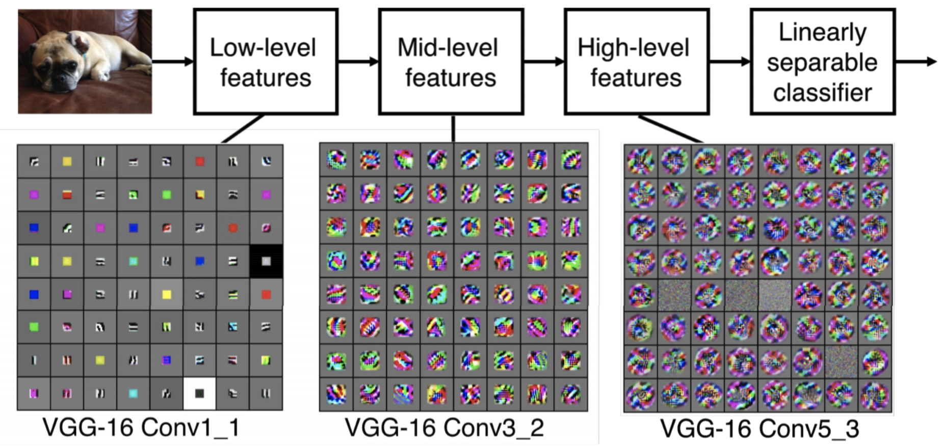
• As the networks becomes deeper, the model learns more complex features. The below is a nice example of this:

In each layer of the CNN, we control a couple of parameters:

• Filter Size: This is the size of filter which we are convoluting over the image
• Number of filters: Weights are not shared between filters, and this determines the depth (# of feature maps) that are output from the layer
• Stride: This defines how many pixels to move over before doing another convolution. This is so that we’re not convoluting over the same pixel an excessive amount of times, as there is some overlap. This also influences the dimensions of the output feature maps
• Padding: This is where we pad some data to the outside of the image. This is for situations when we want to preserve the image dimensions after max-pooling. Also, this can be used if we wanted to prevent the shrinking of our original spatial dimensions. Here is a good example:

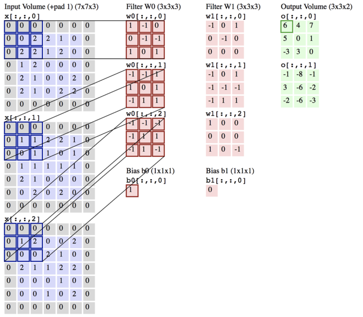
Mathematically, what is the size of the output feature maps? Consider, if we had input size: $m$ x $n$ x $c$, and filter size: $a$ x $b$, stride size: $s$ x $t$, and padding size: $p$ x $q$. What would this entail?

• We pad $p$ pixels on the left/right and $q$ pixels on top/bottom
  • Typically though, we would pad equally on all 4 sides, meaning $p$ = $q$
• Filter size is $a$ x $b$ x $c$. Why? Because the incoming input is $m$ x $n$ x $c$. That is, the input is feature maps, where each map is dimension $m$ x $n$. Then, the depth is $c$. Consider the following diagram explanation:
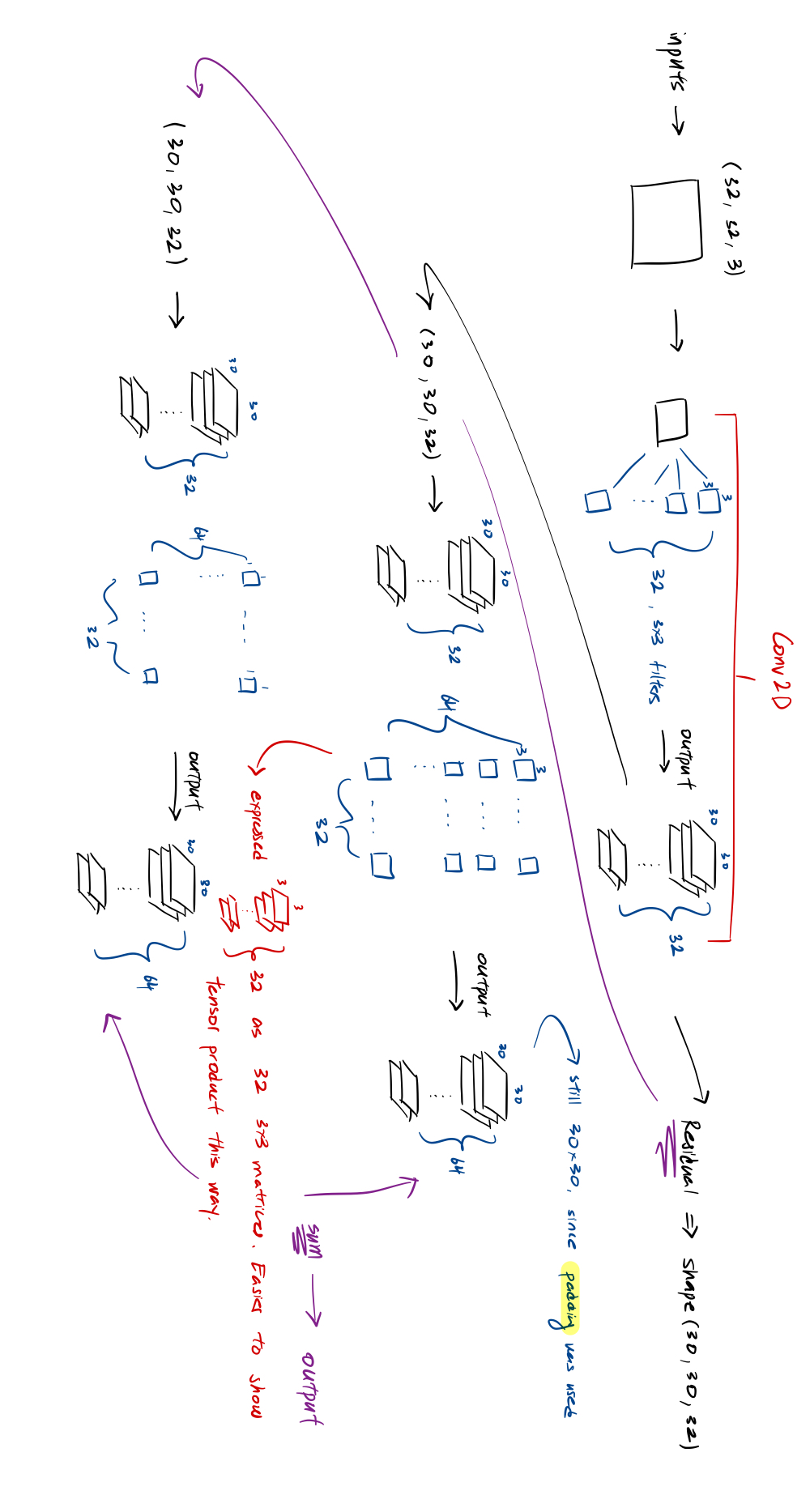
• IMPORTANT: In the first line, for those 32 3 x3 filters, each individual filter, is a tensor (3,3,3). So, each filter (3,3,3) when convoluted against (32,32,3), produces a tensor
• We will move $s$ pixels horizontally and $t$ pixels vertically
• Output size: $\lfloor 1+\frac{m+2p-a}{s}\rfloor$ x $\lfloor 1+\frac{n+2q-b}{t}\rfloor$
• With $p=\lceil \frac{m(s-1)+a-s}{2}\rceil$ and $q=\lceil \frac{n(t-1)+b-t}{2}\rceil$, output size = input size

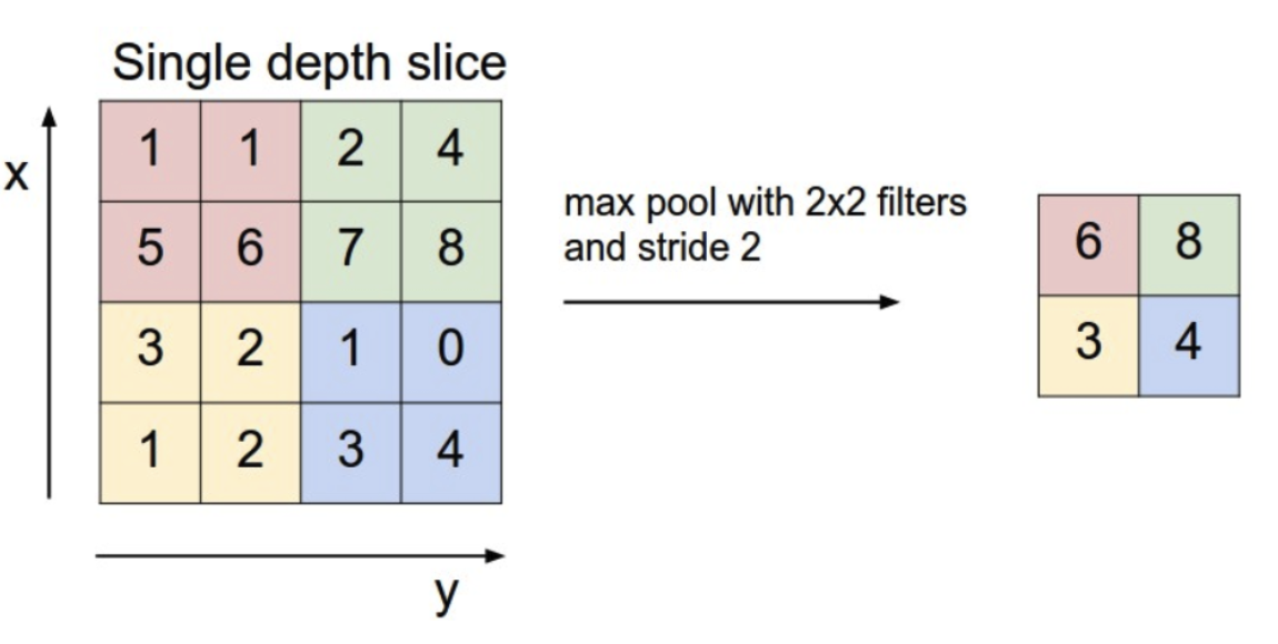
Pooling

This concept should be very familiar, and the below diagram is sufficient:

Architecture

So the idea of what a convolutional layer does, is fairly straightforward. There have been many architecture patterns created over the years. We will take a look at some of them via diagrams.

→ LeNet

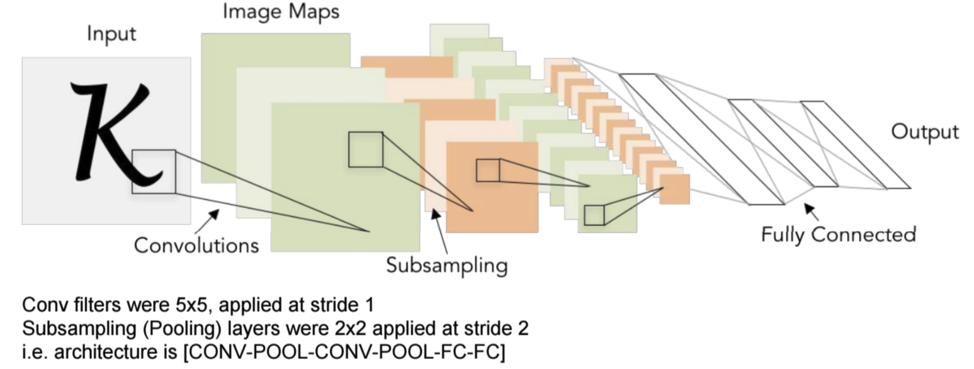
This one is simple: a couple of convolutional layers followed by a sequence of dense layers which are responsible for learning the mapping between feature and label

→ AlexNet

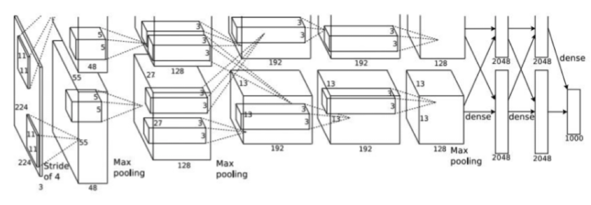
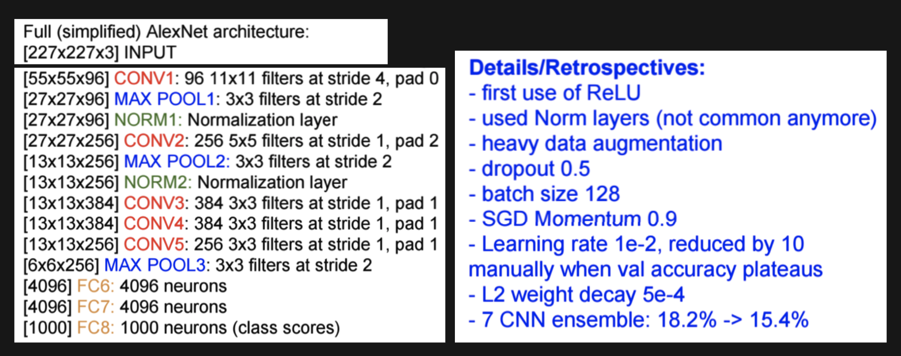
• Similar design, pay attention to the numbers being used. AlexNet is famous for being one of the first convolutional architectures to display very promising results in competitions. It won the ImageNet Large Scale Visual Recognition Challenge in 2012, marking a breakthrough in deep learning. It employs the classic 3x3 kernel dimensions, with 128 depth on the filters and using max-pooling. As seen above, this is not a very deep model and demonstrates the power of CNN’s.
• In addition, we are using ReLU (Rectified Linear Unit), which became one of the most used activation functions
• Heavy data augmentation (don’t want same image trained twice, augment in a data pipeline before next iteration)
• Utilized L2 regularization to improve generalization power

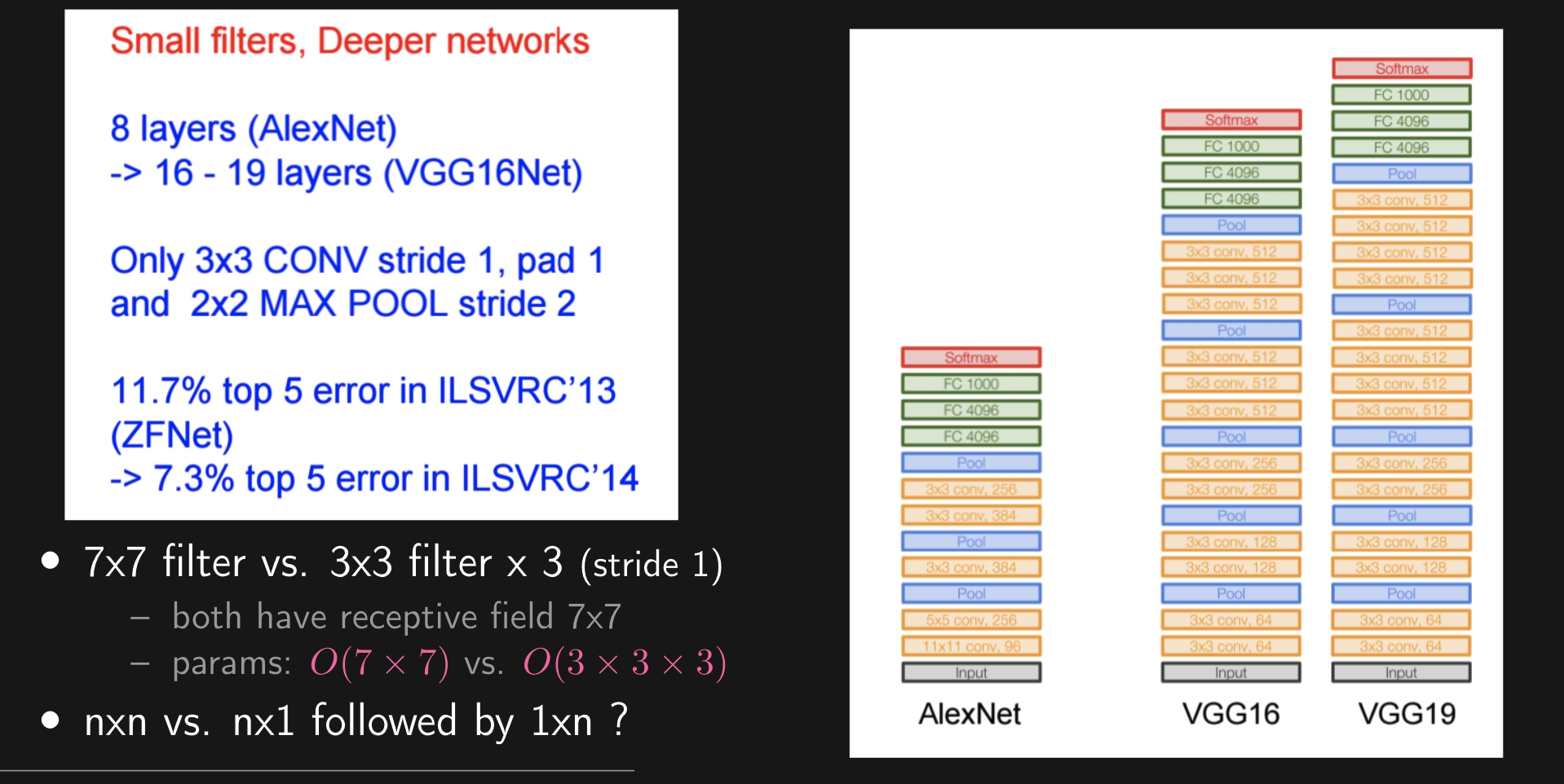
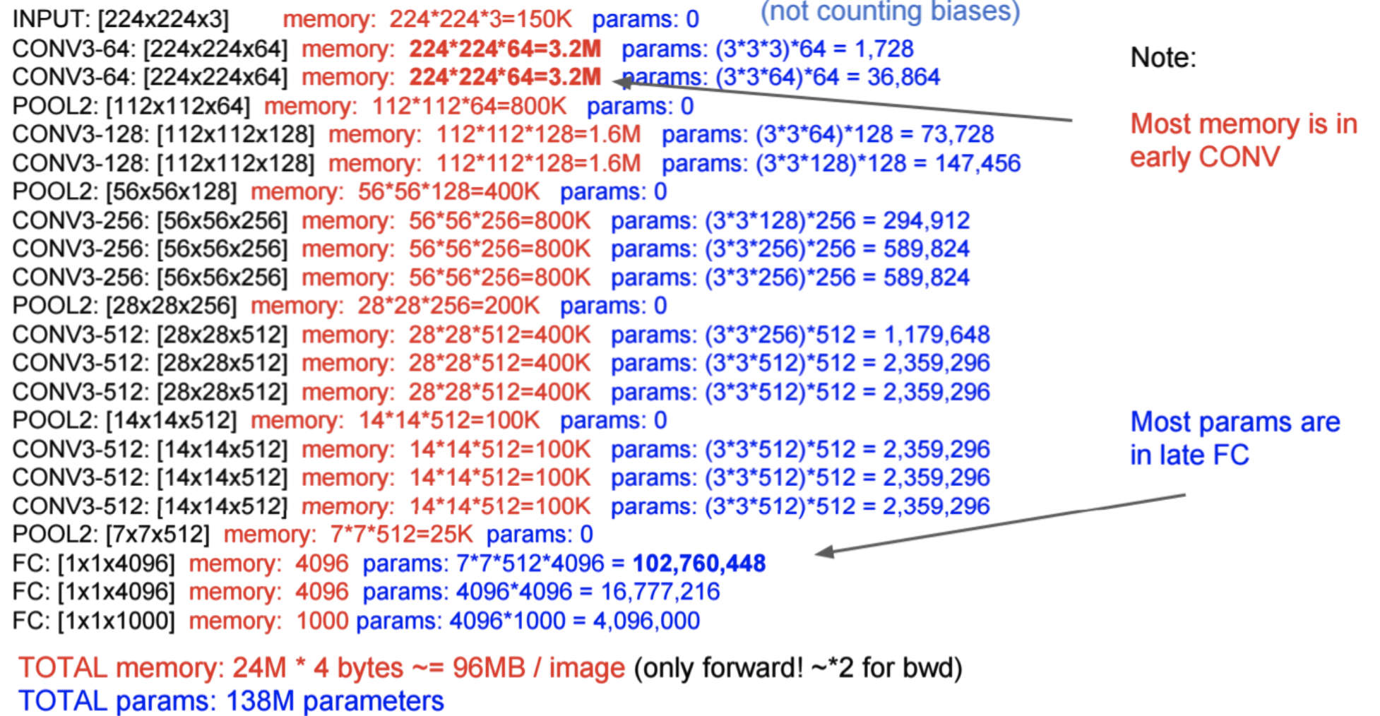
→ VGGNet Another very famous CNN architecture. This is a much larger model than previous ones. It is an architecture known for its simplicity and effectiveness. VGGNet has left a lasting impact on image recognition tasks and has become a benchmark for understanding deep neural networks.

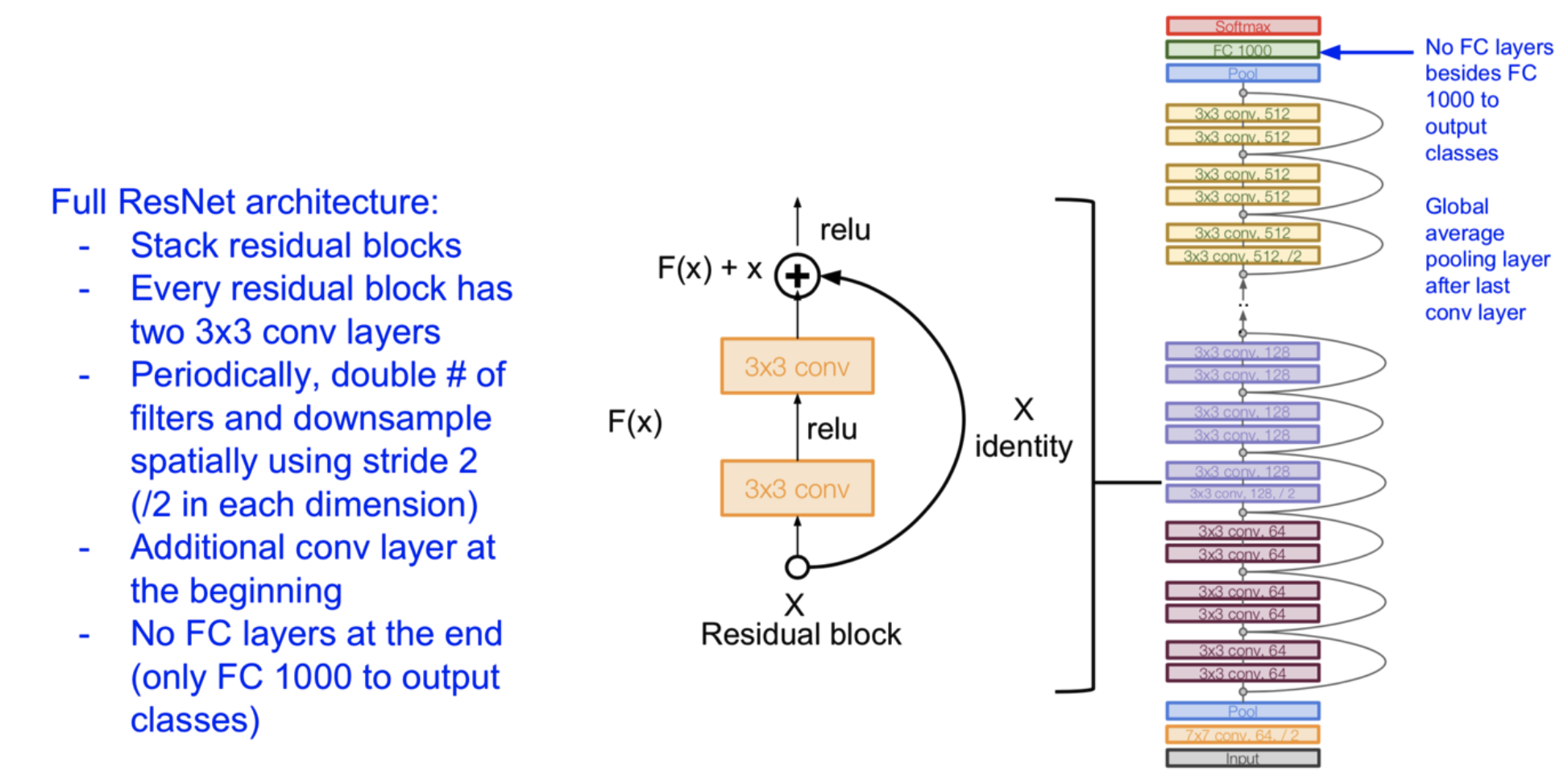
Deeper the Better Deeper models are harder to train due to vanishing / exploding gradient. To see more of this, check Deep Learning Notes. Same for Residual Networks, which help to prevent the “forget” of learned relationships through a residual connection:

• Add a shortcut connection that allows “skipping” one or more layers
• Effectively turning the block into learning residual: output - input
• Allows more direct backpropogation of the gradient through the “shortcut”
• Can also concatenate or add a linear layer if dimensions mismatch