Chapter 4- Getting started with NN- Classification and Regression

Getting started with neural networks: classification and regression

To get this chapter started, we will look at one of the simplest kinds of machine learning problems: binary classification. To learn this, we will create an example of classifying movie reviews as either positive or negative, based on the text context of the reviews. First, let’s load the IMDB data set:

from tensorflow.keras.datasets import imdb
(train_data, train_labels), (test_data, test_labels) = imdb.load_data(
            num_words=10000)

Here, The variables train_data and test_data are lists of reviews; each review is a list of word indices (encoding a sequence of words). train_labels and test_labels are lists of 0s and 1s, where 0 stands for negative and 1 stands for positive. The indexes are indices into the dictionary. The num_words=10000only keep the top 10,000 most frequently occurring words in the training data. Rare words will be discarded. This allows us to work with vector data of manageable size. So, all movie reviews with words not in the top 10,000 frequency, are removed.

---

Preparing the Data

Now, we cannot pass a list of integers into a neural network. Each “word” will have different length, and neural network expects to process contiguous batches of data. For this example, we will convert each list of integers into a 10,000 dimensional vector that is all 0’s, except for the indices of the list. This would mean, for instance, turning the sequence [8, 5] into a 10,000-dimensional vector that would be all 0s except for indices 8 and 5, which would be 1s. Then you could use a Dense layer, capable of handling floating-point vector data, as the first layer in your model. Here is how we would do this:

import numpy as np
def vectorize_sequences(sequences, dimension=10000):
    results = np.zeros((len(sequences), dimension))
    for i, sequence in enumerate(sequences):
      for j in sequence:
        results[i, j] = 1.
    return results
x_train = vectorize_sequences(train_data)
x_test = vectorize_sequences(test_data)
 
y_train = np.asarray(train_labels).astype("float32")
y_test = np.asarray(test_labels).astype("float32")

---

Building the model
So now, the input data is vectors, and the labels are scalars (1s and 0s): this is one of the simplest problem setups you’ll ever encounter. A type of model that performs well on such a problem is a plain stack of densely connected (
Dense) layers with relu activation functions. There are 2 key architecture decisions we need to make:

• How many layers to use
• How many units to choose for each layer

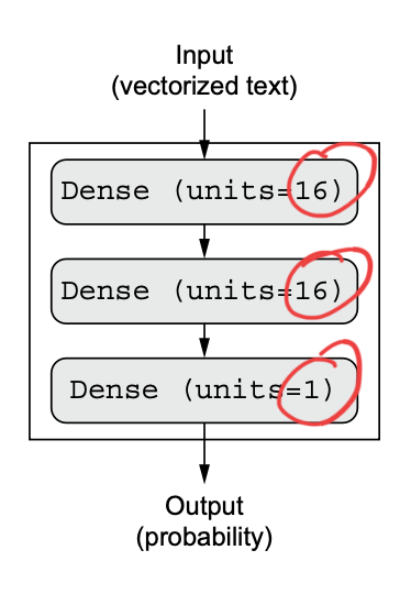
For now, we will use 3 layers, with 2 intermediate layers having 16 units each, and a third layer that will output the scalar prediction regarding the sentiment of the current review.

Why do we do this? We’ll later on learn the reasoning and formal principles to guide us in making these decisions. For the time being, we’ll believe the above is the best solution.

from tensorflow import keras
from tensorflow.keras import layers
model = keras.Sequential([
    layers.Dense(16, activation="relu"),
    layers.Dense(16, activation="relu"),
    layers.Dense(1, activation="sigmoid")
])

Having 16 units means the weight matrix W will have shape (input_dimension, 16): the dot product with W will project the input data onto a 16-dimensional representation space (and then you’ll add the bias vector b and apply the relu operation). You can intuitively understand the dimensionality of your representation space as “how much freedom you’re allowing the model to have when learning internal representations.” Having more units (a higher-dimensional representation space) allows your model to learn more-complex representations, but it makes the model more computationally expensive and may lead to learning unwanted patterns (patterns that will improve performance on the training data but not on the test data).

The final layer uses a sigmoid activation so as to output a probability (a score between 0 and 1 indicating how likely the sample is to have the target “1”: how likely the review is to be positive).

Finally, we need to choose a loss function and an optimizer. Because we’re facing a binary classification problem and the output of your model is a probability (you end your model with a single-unit layer with a sigmoid activation), it’s best to use the binary_crossentropy loss. It isn’t the only viable choice: for instance, you could use mean_squared_error. But crossentropy is usually the best choice when you’re dealing with models that output probabilities.

All of the above information is passed to the model through the compiler:

model.compile(optimizer="rmsprop",
              loss="binary_crossentropy",
              metrics=["accuracy"])

Now, lets set aside a select part of the input data for validation purposes:

x_val = x_train[:10000]
partial_x_train = x_train[10000:]
y_val = y_train[:10000]
partial_y_train = y_train[10000:]

We’ll create a validation set by setting apart 10,000 samples from the original training data.

We will now train the model for 20 epochs (20 iterations over all samples in the train- ing data) in mini-batches of 512 samples. At the same time, we will monitor loss and accuracy on the 10,000 samples that we set apart. We do so by passing the validation data as the validation_data argument.

history = model.fit(partial_x_train,
                    partial_y_train,
                    epochs=20,
                    batch_size=512,
                    validation_data=(x_val, y_val))

Remember that the model.fit() command returns a History object. This object has a member called history, which is a dictionary containing data about everything that happened during training. Let’s look at it:

history_dict = history.history
history_dict.keys()
# [u"accuracy", u"loss", u"val_accuracy", u"val_loss"]

The dictionary contains four entries: one per metric that was being monitored during training and during validation. In the following two listings, let’s use Matplotlib to plot the training and validation loss side by side (see figure 4.4), as well as the training and validation accuracy (see figure 4.5).

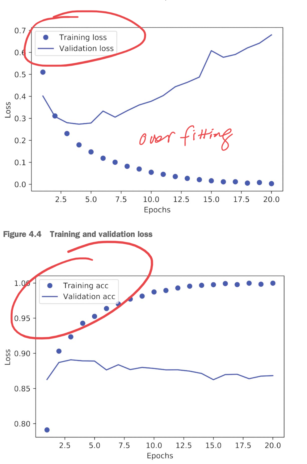
The first one compares loss, the second one compares accuracy (y-axis label is a typo).

We notice the following:

• The training loss decreases with every epoch, and the training accuracy increases with every epoch - what we expect
• But that isn’t the case for the validation loss and accuracy: they seem to peak at the fourth epoch

The above example demonstrates an example of over-training. The model has now “memorized” the training data, and ineffective on new data, which is what the goal of machine learning is. In this case, after the 4th epoch, we have begun to over optimize on the training data, and the model has ended up learning representations that are specific to the training data, and don’t generalize outside of training data.

In this case, to prevent overfitting, you could stop training after four epochs. In general, you can use a range of techniques to mitigate overfitting, which we’ll cover in chapter 5. Let’s create a new model for 4 epochs and train it:

model = keras.Sequential([
    layers.Dense(16, activation="relu"),
    layers.Dense(16, activation="relu"),
    layers.Dense(1, activation="sigmoid")
])
 
model.compile(optimizer="rmsprop",
              loss="binary_crossentropy",
              metrics=["accuracy"])
model.fit(x_train, y_train, epochs=4, batch_size=512)
results = model.evaluate(x_test, y_test)
# results is >> [0.2929924130630493, 0.88327999999999995], first is test loss and the second is test accuracy

Quick Summary:

• You usually need to do quite a bit of pre-processing on your raw data in order to be able to feed it as tensors into a neural network
• Stacks of Dense layers with relu activation functions can solve a wide range of problems (including sentiment classification), and you’ll likely use them frequently.
  • Recall that a Dense layer with a relu (rectified linear unit function) performs: output = relu(dot(input, W) + b)
• In a binary classification problem (two output classes), your model should end with a Dense layer with one unit and a sigmoid activation: the output of your model should be a scalar between 0 and 1, encoding a probability.
• With such a scalar sigmoid output on a binary classification problem, the loss function you should use is binary_crossentropy.
• The rmsprop optimizer is generally a good enough choice, whatever your problem. That’s one less thing for you to worry about.
• If we train too much, we run the risk of over-training and eventually, become increasingly worse on data sets they have never seen before

---

Now, we look at something similar: a multi-class classification example. This is largely the same as the binary classifier. The only differences are in the activation functions we may choose to use as well as the loss function and output of the model.

---

Lastly, we will look at regression. Another common type of machine learning problem is regression, which consists of predicting a continuous value instead of a discrete label: for instance, predicting the temperature tomorrow, given meteorological data or predicting the time that a software project will take to complete, given its specifications.

For this example, we will train a model on a set of Boston market housing data from the 1970’s. The first thing to know is the shape of the data. For this data set, there are only 506 data samples, being split into 404 training samples and 102 test samples. Here is what the data is like:

>>> train_data.shape
(404, 13)
>>> test_data.shape
(102, 13)

Each sample has 13 numerical features, which represent things such as per capita crime rate, average number of rooms per dwelling, accessibility to highways, and so on. The targets are the valuations of the homes (in thousands of USD)

>>> train_targets
[ 15.2,  42.3,  50. ...  19.4,  19.4,  29.1]

Now, for neural networks, its a bit problematic to feed it these 13 values that are of such different ranges. A widespread best practice for dealing with such data is to do feature-wise normalization: for each feature in the input data (a column in the input data matrix), we subtract the mean of the feature and divide by the standard deviation, so that the feature is centred around 0 and has a unit standard deviation. This is easily done in NumPy:

mean = train_data.mean(axis=0)
train_data -= mean
std = train_data.std(axis=0)
train_data /= std
test_data -= mean
test_data /= std

As the number of samples is not a lot, we will only use 2 hidden layers. The last layer will not have an activation function. The model ends with a single unit and no activation (it will be a linear layer). This is a typical setup for scalar regression (a regression where you’re trying to predict a single continuous value). The output can be anything, and we don’t want restrict that with an activation function.

def build_model():
  model = keras.Sequential([
      layers.Dense(64, activation="relu"),
      layers.Dense(64, activation="relu"),
      layers.Dense(1)
  ])
 
  model.compile(optimizer="rmsprop", loss="mse", metrics=["mae"])
  return model

So, notice that we are now using "mse" and "mae" as our respective loss function and metric.

• Note that we compile the model with the mse loss function — mean squared error, the square of the difference between the predictions and the targets. This is a widely used loss function for regression problems.
• We’re also monitoring a new metric during training: mean absolute error (MAE). It’s the absolute value of the difference between the predictions and the targets. For instance, an MAE of 0.5 on this problem would mean your predictions are off by $500 on average.

We do not have a lot of data samples, and if we were to cut a sample from the training data to use a validation data, it would be very small. As a consequence, the validation scores might change a lot depending on which data points we chose for validation and which we chose for training: the validation scores might have a high variance with regard to the validation split. This would prevent us from reliably evaluating our model. In situations like this, the best practice is to use K-fold cross-validation.

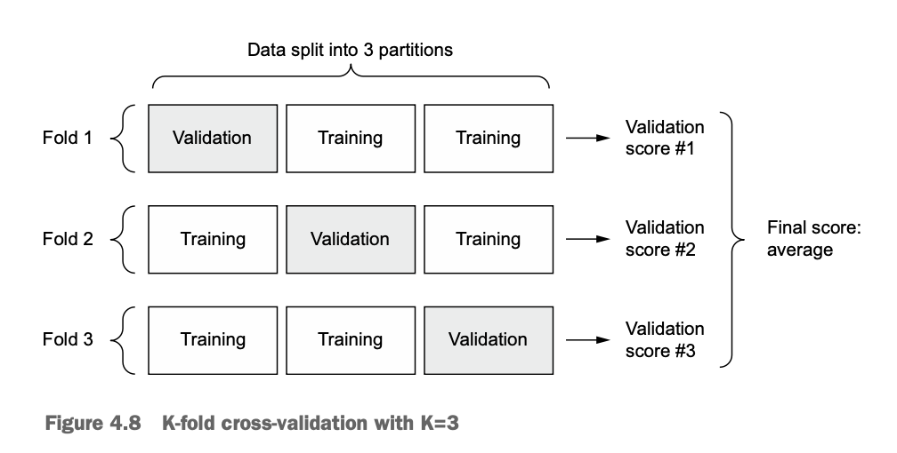
The idea of how it works is fairly simple. We will create k partitions (k-fold). Then, we loop through it k times, each time, choosing a different block of data to be the validation data, and the rest — training data. After all k iterations, we ill take the mean of the validation scores. Here is the code for this:

for i in range(k):
  print(f"Processing fold #{i}")
  val_data = train_data[i * num_val_samples: (i + 1) * num_val_samples]
  val_targets = train_targets[i * num_val_samples: (i + 1) * num_val_samples]
 
  partial_train_data = np.concatenate(
    [train_data[:i * num_val_samples],
     train_data[(i + 1) * num_val_samples:]],
    axis=0)
 
  partial_train_targets = np.concatenate(
      [train_targets[:i * num_val_samples],
       train_targets[(i + 1) * num_val_samples:]],
      axis=0)
 
  # the below is not related to the fold anymore, just building, fitting, and seeing how more epochs impacts effectiveness (can see when overtrain)
  model = build_model()
 
  history = model.fit(partial_train_data, partial_train_targets,
                      validation_data=(val_data, val_targets),
                      epochs=num_epochs, batch_size=16, verbose=0)
 
  mae_history = history.history["val_mae"]
  all_mae_histories.append(mae_history)

For this model, we initially train it for 500 epochs, which we will notice is to much. We know that the keras .fit() method returns a history object. It contains information about the training process and the metrics recorded during training. For instance:

• loss: The training loss values for each epoch.
• val_loss: The validation loss values for each epoch (if validation data is provided).
• mae: The mean absolute error (MAE) values for each epoch on the training data.
• val_mae: The MAE values for each epoch on the validation data (if validation data is provided).

We will see how this model performs best at 130 epochs, and after that, becomes to over-train.

• Yes, after each fold in k-Fold Cross-Validation, the model weights are typically reset or reverted back to their original values before training on the next fold. This is important to ensure that the model starts each iteration with the same initial conditions and does not carry information learned from one fold to the next.

---

→ Summary:

• The three most common kinds of machine learning tasks on vector data are binary classification, multi-class classification, and scalar regression.
• You’ll usually need to pre-process raw data before feeding it into a neural network.
• When your data has features with different ranges, scale each feature independently as part of pre-processing.
• As training progresses, neural networks eventually begin to over-fit and obtain worse results on never-before-seen data.
• If you don’t have much training data, use a small model with only one or two intermediate layers, to avoid severe over-fitting.
• If your data is divided into many categories, you may cause information bottlenecks if you make the intermediate layers too small (units/neurons)
• When you’re working with little data, K-fold validation can help reliably evaluate your model.