Chapter 4- Kernels

Overview

Kernels are especially needed when we are dealing with non-linearly separable data and non-linear data. Consider the following situation:

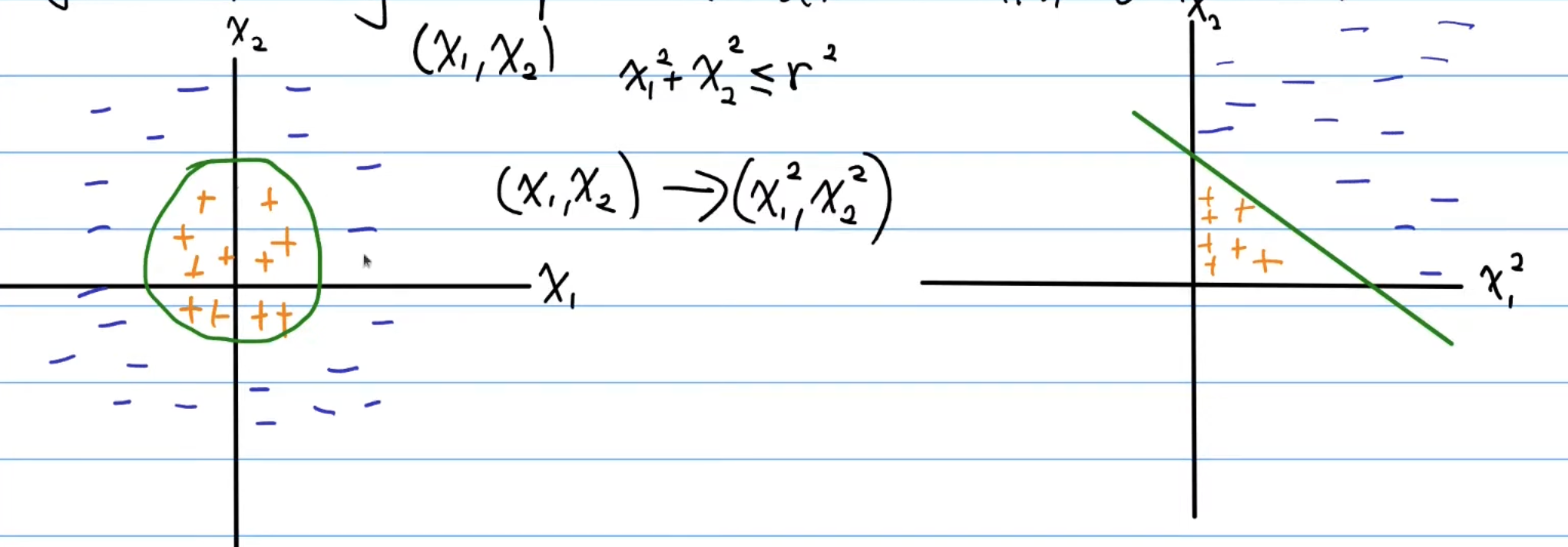
Now, the data on the left cannot be classified using a hyperplane, since the decision boundary is non-linear. We notice that if we were to draw one, one reasonable idea is it to just draw a circle around the data, with the equation of the circle. Now, let’s apply a non-linear transformation to the data. This function $\varphi :{\mathbb{R}}^2\to {\mathbb{R}}^2$, transforms the left data points into the right, which is now linearly separable. Ok, thats cool, but same dimension transformations aren’t always feasible like this. A classic example of this is XOR:

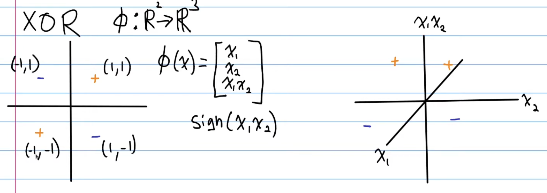
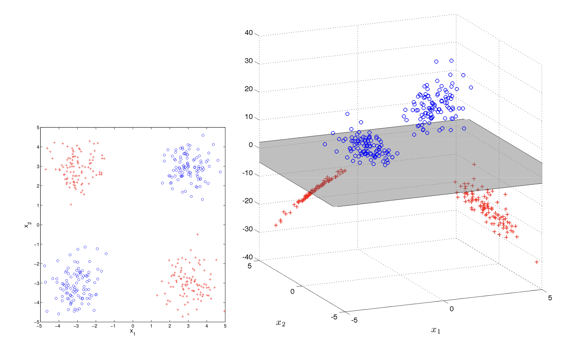
Now, there is no such linear transformation in the same vector space, that will transform our data into a linearly separable format. Instead, we need to increase the dimension of the data set. Consider the XOR Problem in the above. For each point we apply a linear transformation $\varphi :{\mathbb{R}}^2\to {\mathbb{R}}^3$, where $(x_1,x_2)\to [x_1,x_2,x_1\cdot x_2{]}^T$. Now, we map each 2D data point into the 3-dimensional space. Notice that the last value of the vector is determines the vertical height of the point, with positive being above the $x_1{x}_2$ plane and negative being below. Now, we can draw a hyperplane as a decision boundary and once again, our dataset is linearly separable.

In kernel methods, what we are really interested in is the phi ($\varphi$) function, which defines the non-linear transformation being applied. We call this feature maps.

Feature Maps

Consider $x\in {\mathbb{R}}^d,y\in \{\pm 1\}$

So we’re looking to transform $x$, most likely to some higher dimension, and we’ve actually already kind of done this when we were concatenating our bias term to the model weight for simplicity in notation. So, we could think of it like: $\varphi (x)=[x,1{]}^T,W=[P,b]\in {\mathbb{R}}^{d+1}$, where $P$ is the previous weight before concatenating. Then, in perceptron and also SVM, our classifier was computed via this $⟨\varphi (x),W⟩>0$. This is the exact idea of feature maps. So, given some data, we are going to map $x\to \varphi (x)$ and $P\to W$.

• So, expanding this dot-product in the above, we get: $⟨\varphi (x),W⟩=x^{T}P+b>0$

• This is the most basic feature map, but this isn’t very expressive as this is a linear transformation of the data points (merely elevating it to $z=1$ in 3-dimensional space).

• As seen in the very first example, we need a non-linear transformation.

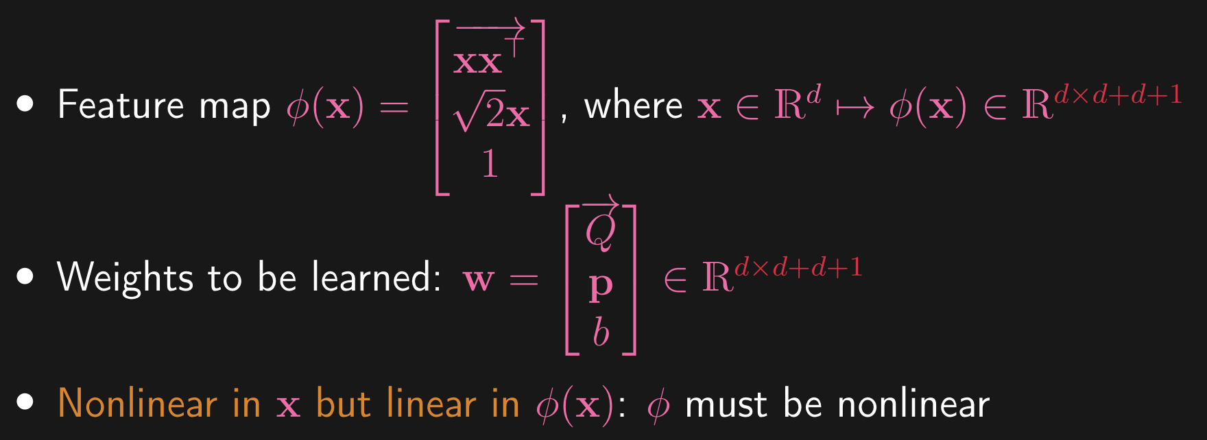
What if we want a more expressive type of classifier? Something like: $⟨x,Qx⟩+\sqrt{2}⟨x,P⟩+b>0$. What is this? This is another type of feature map called a quadratic classifier. So, for this what are the model weights?

• $b\in \mathbb{R}$ is our constant bias, as usual

• $P\in {\mathbb{R}}^d$ is our vector weight

• $Q\in {\mathbb{R}}^{dxd}$ matrix weight with more parameters

• Why do we use $\sqrt{2}$ ? This is just a scaling factor, and so does not change the problem by much, we’ll see later on why we choose this scaling factor.

So this is the form of the classifier that is more expressive than the first example. Let’s simplify this, as we want to write this as the inner-product of some sort of feature map and some sort of parameter vector (we want something that resembles $⟨\varphi (x),W⟩$. Let’s first expand $⟨x,Qx⟩$:

$⟨x,Qx⟩$

Note that in the above, Now, we can re-arrange this lengthy summation expression. Namely:

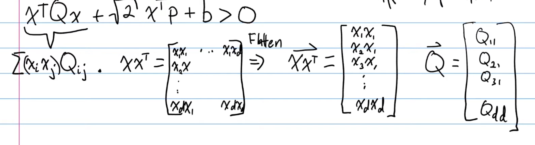
When we flatten, we are stacking the column vectors of the the matrix on top of each other, forming a ${\mathbb{R}}^{d^2}$ vector. So, the above summation can be expressed as $⟨x,Qx⟩=x^{T}Qx=⟨\overrightarrow{x{x}^T},\vec{Q}⟩$. Now, we can write the quadratic classifier as the inner product of a feature map and parameter vector:

Where again, we’re stacking these vectors vertically to create new higher dimension vectors. So, the quadratic classifier becomes $⟨\varphi (x),W⟩$. Now, the feature map blows up the dimension, as we are performing a $\varphi :{\mathbb{R}}^d\to {\mathbb{R}}^{d^2+d+1}$ transformation.

==Computation==

Something interesting to note is the time complexity of such an action, as squaring the dimensionality of data could substantially increase runtime, and thus take much more resources to compute such a model. For example, consider the set of data before the transformation. In that case, computing inner product of weight and data, would be $O(d)$. Now, our weight and data have been exponentially increased in expressiveness. So, if we computed the same thing, the runtime would be $O(d^2)$, and potentially much much more costly if we had more complex feature map (could easily skew towards $\infty$, which is often the case when working with real world data). Is this always the case?

• The good news is, this computation can be done much more efficiently

• To see this well, let’s revisit the SVM dual problem

Consider:

\begin{array}{ll}

==Notice that in the above, we have now added phi to the data points==. Now, we know:

$\varphi (x)=\left(\begin{array}{c}\overrightarrow{x{x}^T}\\ \sqrt{2}x\\ 1\end{array}\right)$

So, if we compute $⟨\varphi (x),\varphi (x^{\prime })⟩$ naively, then we would need $O(d^2)$ time. But, observe:

$⟨\overrightarrow{x{x}^T},\overrightarrow{x^{\prime }{x}^{\prime T}}⟩+⟨\sqrt{2}x,\sqrt{2}{x}^{\prime }⟩+1$ is the above inner product. We can further simplify this into:

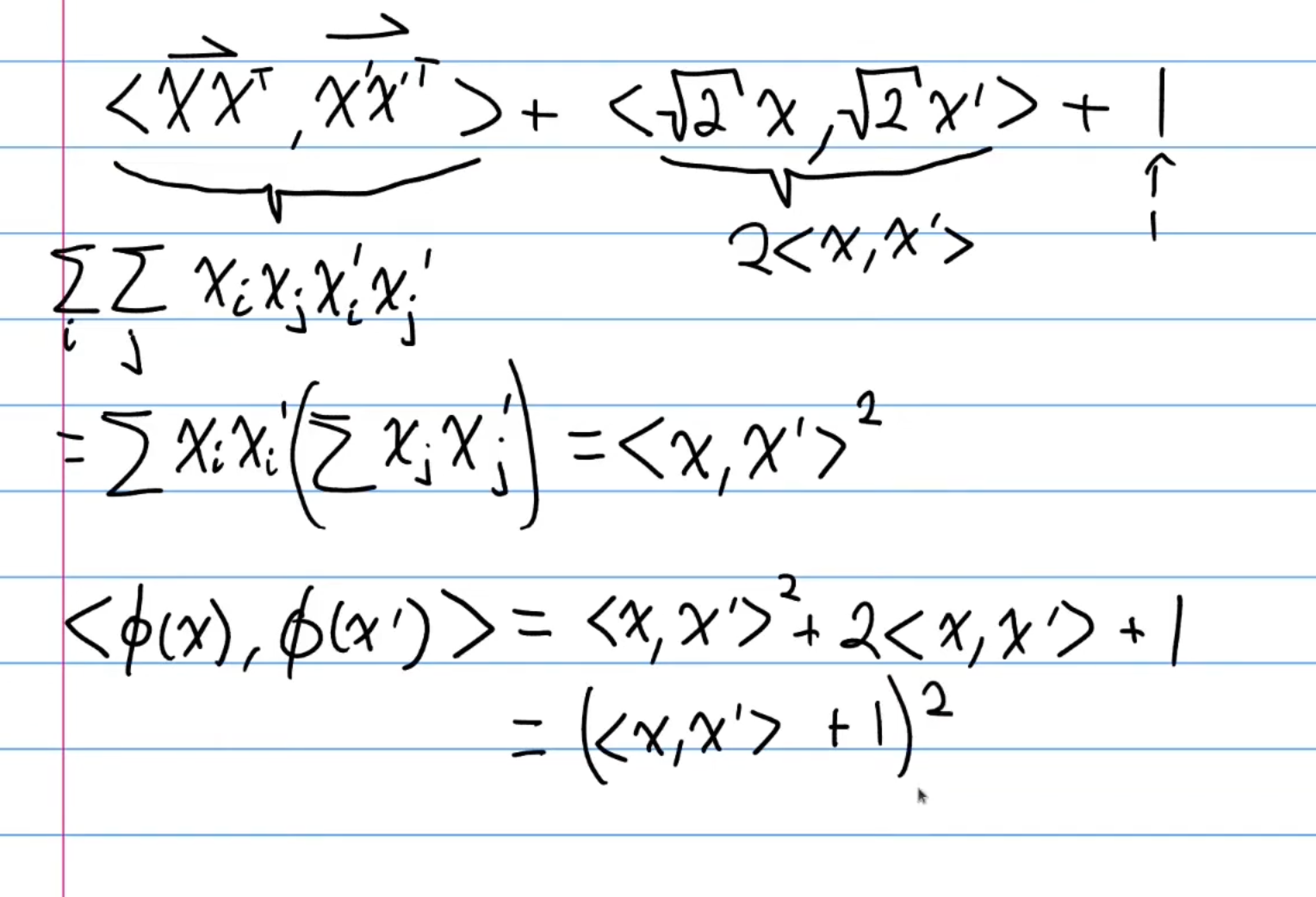
Now why is this useful? As seen, we only need to compute inner product between the 2 data points $x,x^{\prime }$, and operate in the d-dimensional space instead of $d^2+d+1$ space, hence making our computations run in $O(d)$. ==This notion is the idea of a reproducing kernel==, the main focus of this chapter, that is, there exists some function $k$, that computes out feature mapped inner product in $d$ dimensional space.

Kernel

We call $k:{\mathbb{R}}^d\text{ x }{\mathbb{R}}^d\to \mathbb{R}$ a kernel if there exists some feature map $\varphi :{\mathbb{R}}^d\to {\mathbb{R}}^H$ (some higher dimension, usually) such that $⟨\varphi (x),\varphi (x^{\prime })⟩=k(x,x^{\prime })$, i.e a simple way to represent the inner product of the feature maps of any 2 vectors. This is especially useful in sitations when $\varphi (x)$ is incredibly high dimension, and would then take incredible computation time, but $k$ is not.

Now, we are familiar with 2D and 3D vector spaces, where operations like inner and outer product are defined. Now, generalizing this to higher dimensions, we call this a Hilbert Space. Think of a Hilbert space as an extension of our usual spaces to infinite dimensions, equipped with tools (like the inner product) to measure lengths and angles, and ensuring that all expected limits are included in the space.

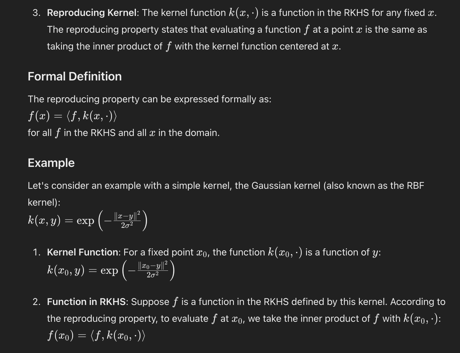
==→ Reproducing Kernel Hilbert Space (RKHS)==

3 main points:

• This is a special kind of Hilbert space (A Hilbert space is a space on which an inner product is defined, along with an additional technical condition) that is associated with a kernel function.
• The space is associated with a kernel function $k(x,y)$, which is a positive definite function. This kernel function defines the inner product in the RKHS.
• Reproducing property:

  • The reproducing kernel $k(x,y)$ has the property that for any function $f$ in the RKHS and any point x in the domain, the value $f(x)$ can be computed as $f(x)=⟨f,k(x,\cdot )⟩f(x)=⟨f,k(x,\cdot )⟩$

  • But what does this mean? I don’t know lmao. Here’s some stuff that might help:

    

  • Visual Intuition: Imagine a set of functions $f$ living in a space defined by the kernel. Each function can be “probed” at any point $x$ by taking an inner product with the kernel function centred at $x$. This probing gives us the value of the function at that point.

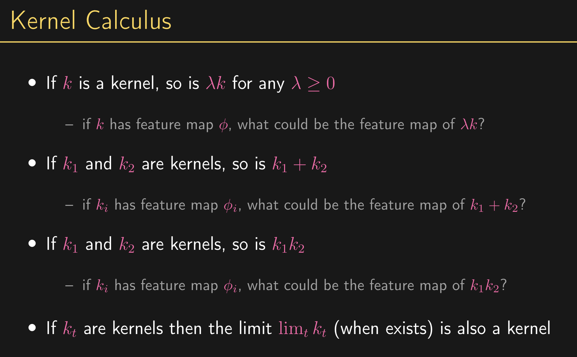
==→ What makes a valid kernel?==

So, what kind of kernels correspond to feature maps? There are certain properties that are needed to characterize which functions are kernel functions.

Take any set of data points $x_1,x_2,...,x_n$, and let $K_{ij}=k(x_i,x_j)\in {\mathbb{R}}^{nxn}$. So, we start with some dataset and we compute the kernel for every pair of points in the dataset, and we store all of these in a matrix. There are some properties we need on this matrix:

1. Symmetric: That is, $K_{ij}=K_{ji}$

2. Positive Semi-definite: Which means we have the following property: $v^{T}Kv>0$ for all $v\in R^n$

   

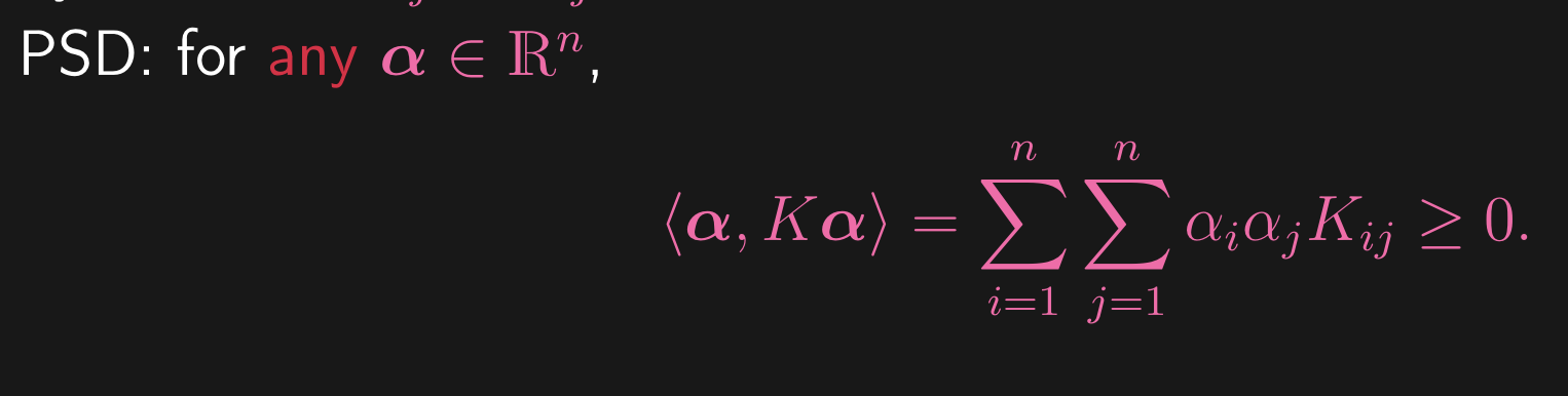
If the 2 properties hold, no matter what data set we feed into it, then it is a valid kernel, where it corresponds to some feature map.

==→ Examples of Kernels==

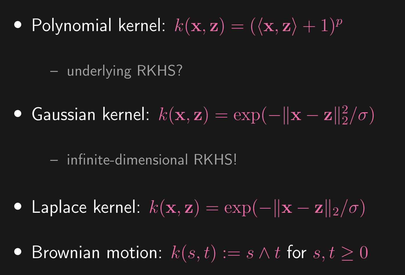
Using Kernels in SVM

Again we revisit the SVM dual objective function:

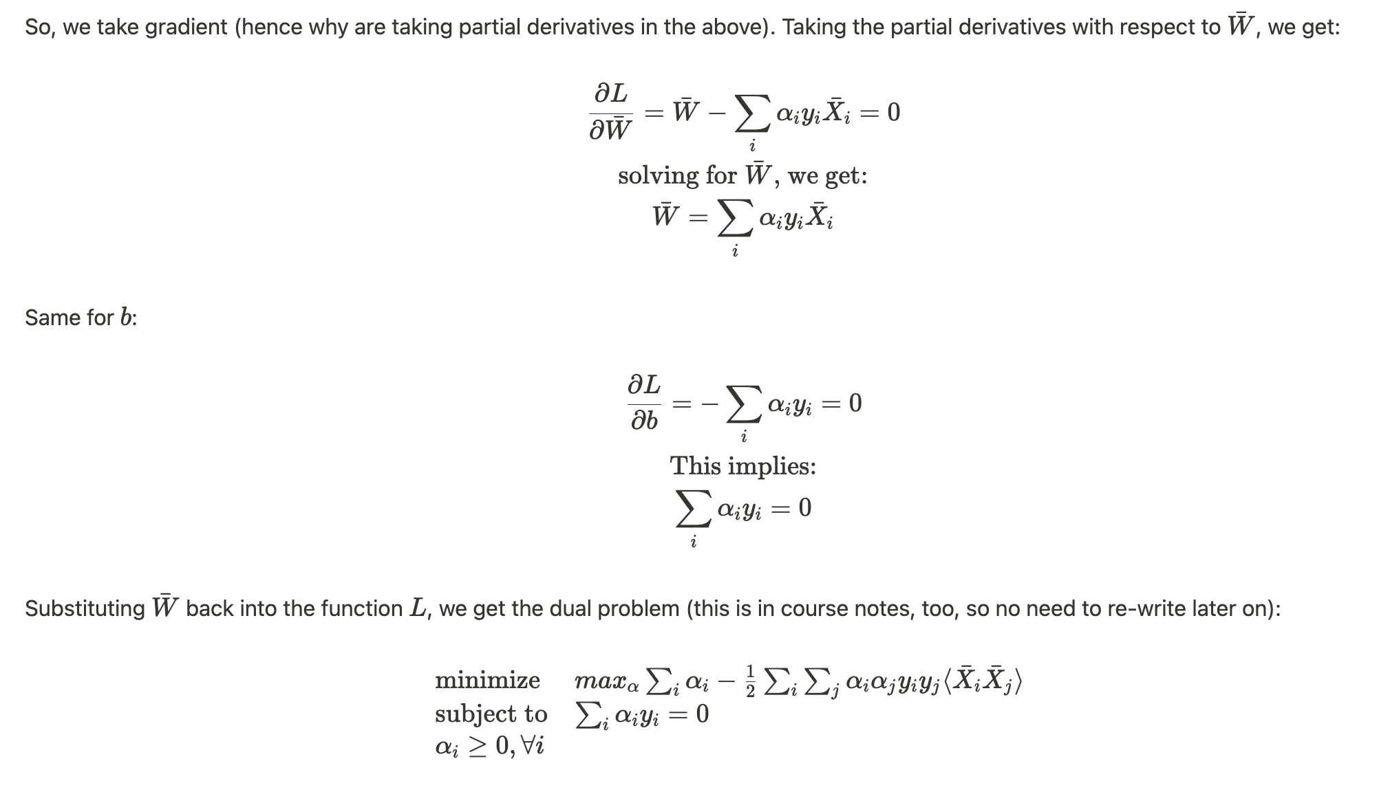
This was the derivation we see in SVM lecture. We use it now. So, as seen, we computed the inner product of the 2 data points. Given the $K$ matrix we defined above. So, this is effectively:

\begin{array}{ll}

Now, we know that $K_{ij}=⟨\varphi (x_i),\varphi (x_j)⟩=k(x_i,x_j)$ our kernel function. Ok, so with this, we can express our vector weight as:

$w=\sum {\alpha }_i{y}_i\varphi (x_i)$

Now, as we’ve stated before, $\varphi (x_i)$ is too high dimension, and we want to look for better way to do this. This means $w$ may be also a too high dimension vector as well. Remember that SVM classifies by:

$sign(⟨w,\varphi (x)⟩)=sign(\sum {\alpha }_i{y}_i⟨\varphi (x_i),\varphi (x)⟩)=sign(\sum {\alpha }_i{y}_{i}k(x_i,x))$

So, we don’t need to necessarily compute $w$ directly, rather, upon expanding, the operation is $O(d)$.

→ Computations for SVM / Tradeoffs

• Linear Kernel: training is $O(nd)$ over $n$ in dataset, and testing is $O(d)$
• General Kernel: training is $O(n^{2}d)$ and testing is $O(nd)$
  • Why? Well the test set is easy to see. Upon a single inner product between weight and data point, we have: $sign(\sum {\alpha }_i{y}_{i}k(x_i,x))$. Now, the kernel component is $O(d)$ time as that is the dimension the data point. Then, we sum this over all points in the training set which have ${\alpha }_i>0$, and that is in the worst case where everything is support vector, $O(n)$ kernel computations → $O(nd)$.
  • This is a fairly large cost, but much better than naively trying to compute the the higher dimension inner products in general