Chapter 2- Linear Regression

Let’s first start off with what is regression. Broadly, regression is a practice used to analyze the relationships between variables, specifically and independent variable and a dependent variable. When we perform regression in machine learning, we are, given a dataset, trying to predict future values. For example, say we have are trying to predict housing data from some other data such as crime rate, education etc. Solving this problem is regression, and we will see in this chapter, how we can create models to predict on this for us.

💡 Idea: Given a training data $(x_i,y_i)$, find a function $f:X\to Y$, such that $f(x_i)\approx y_i$ where

1. $x_i\in {\mathbb{R}}^d$: the feature vector for the $i^{th}$ training example
2. $y_i\in Y\subseteq {\mathbb{R}}^t$: $t$ responses

So, each data point is some vector, and the response, could be anything from a simple scalar value (think predicting something like stock price), to higher dimension vectors (perhaps we’re predicting multiple traits).

• In theory, for any finite training data set, there exist an infinite number of functions $f$ such that for all $i$, we have $f(x_i)=y_i$. Consider something like:

  

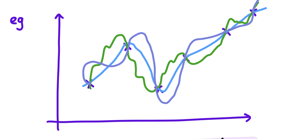
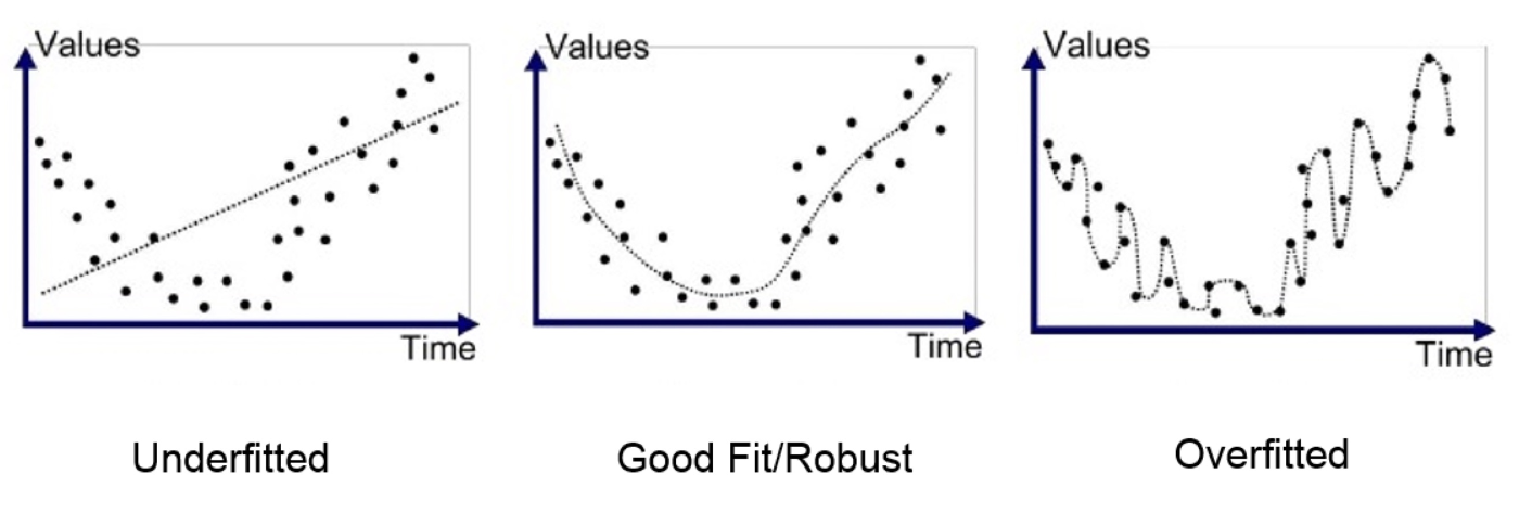
• So, we must be careful about how we fit our model/function to the data. Unlike in classification tasks as simple as perceptron, where 100% accuracy on training data is normal, we don’t want our model to perform exceptionally well on our training data. Here are some examples of functions found after training to a training data set:

  

• What do we see here? If we find a function, that does indeed correctly and precisely predict in our training set, chances are, it has poor generalization, which defeats the entire purpose of machine learning in the first place. This thought process is reflected in all aspects of deep learning, and especially will become important topics upon learning more powerful models.

$m$ is our optimal function. That is, it is the best possible $f(x)$ function, as it we know:

$m(x)=\underset{f:X\to Y}{\min }E\Vert f(X)-Y{\Vert }_2^2$

Here, $m$ is the theoretical regression function, the function that minimizes the expected squared error between the predictions $f(X)$ and the actual values $Y$. Of course, $m$ requires us to know the distribution of both $X$ and $Y$, which is infeasible for real world data. The goal is to learn an approximation $\hat{f}(x)$ of the true regression function $m(x)$ using the samples in our training set. The primary objective in machine learning is to find the function $\hat{f}(x)$ that generalizes well to new unseen data. One method to improve generalization and reduce over-fitting is cross-validation, which is something we will see later in this chapter.

Before we jump right into how machine learning models learn in regression, its best to start of by considering what characteristics of the regression function should be pay attention to for the model to improve itself. To see this, we need to analyze the error of models. In the above, $f(x)$ is the function our model is predicting, and we want to see at a more granular level, where the error of our model is from. This is why we do bias-variance decomposition, as it helps us to understand the sources of error in our model and guides the model in how to lern and improve in the next training iteration. Here is an derivation of the decomposition:

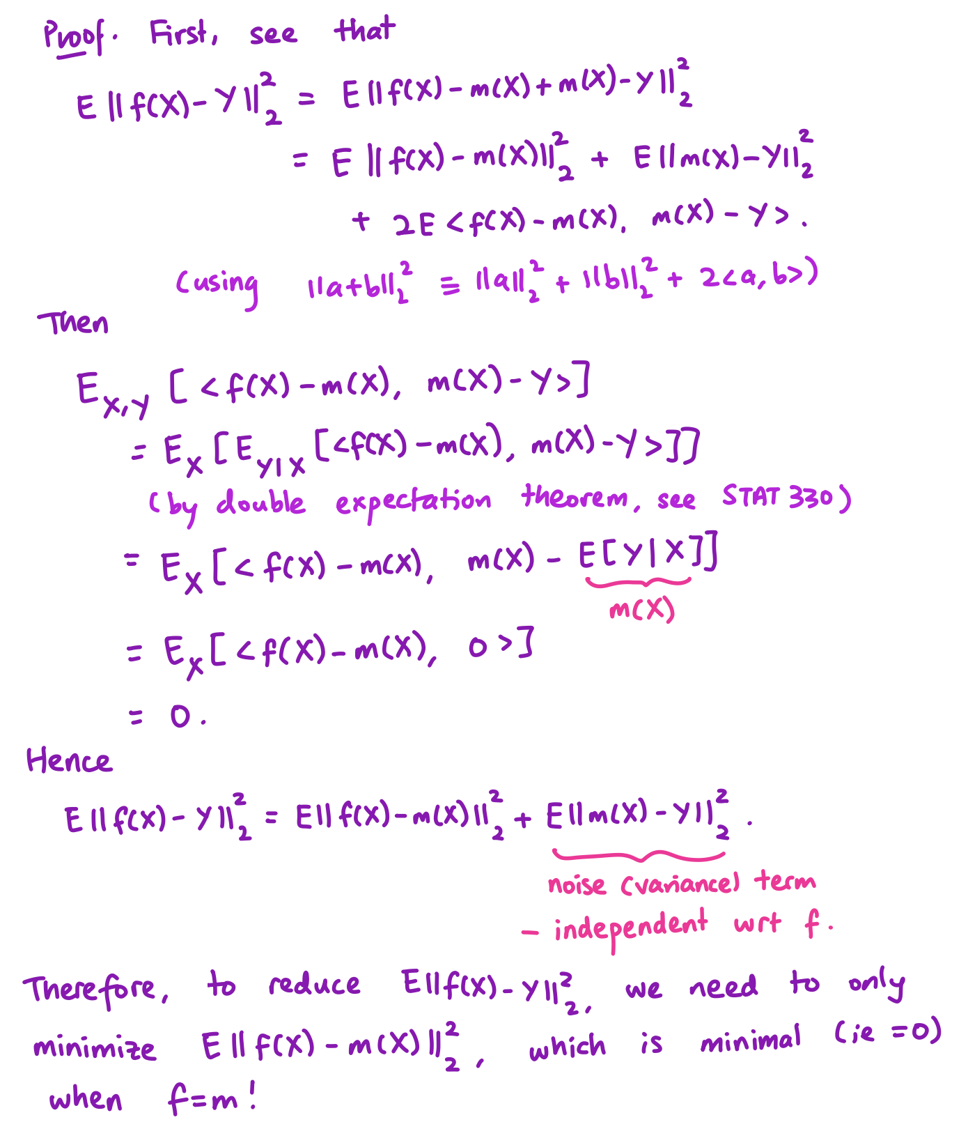
As seen, there 2 components that have surfaced. The noise (variance term) is independent of $f$ and represents the irreducible error inherent in the data. So, to improve our model, we need to minimize the bias${}^2$, hence, the square error between the regression function and our predicted function. How can we do this? If we can get $f(x)$ as close as possible to $m(x)$, we will minimize our error. So, this echos the goal of machine learning in regression: finding function $f$ that approximates $m$.

To do so, we introduce the notation:

$\underset{f:X\to Y}{\min }\hat{E}\Vert f(X)-Y{\Vert }_2^2=\frac{1}{n}{\sum }_{i=1}^n\Vert f(X_i)-Y_i{\Vert }_2^2$

This represents the empirical estimate of the expected error between the model predictions and the true outcomes. This is reflects how well our model $f(x)$ performs on the given dataset in terms of predicting the outcomes $Y$. In ML, we have a sort of lemma, which is:

Uniform Law of Large Numbers: as training data size $n\to \infty$, then our estimate will become closer and closer towards the real value

So, this has been an overview of regression, and an entry into what we are looking to accomplish with linear regression. We’ll look at one(and the most important) example: linear least squares regression

---

Linear Least Squares Regression

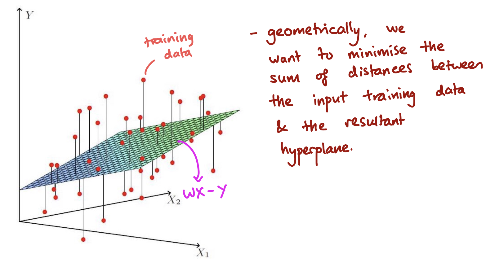
This is the idea of linear regression and we are trying to minimize the squared distance from the the predicted value to the actual value — Least Squares. This is our loss function and the method in which our regression model will learn. Let’s re-introduce some notation moving forward:

→ Linear Least Squares Regression

Our regression functions are affine. They will be of the form:

$f(x)=Wx+b,w\in {\mathbb{R}}^{t\text{ x }d},\text{and }b\in {\mathbb{R}}^t$

where:

• $t$ = # of response parameters we want to predict z3e45rt!Q.
• $d$ = # of input parameters

Again, we can pad our function like before to make it more concise to write:

$x\leftarrow \left(\genfrac{}{}{0ex}{}{x}{1}\right),W\leftarrow [W,b],\text{ hence, }f(x)=Wx$

So, we can express Chapter 2- Linear Regression using matrix form:

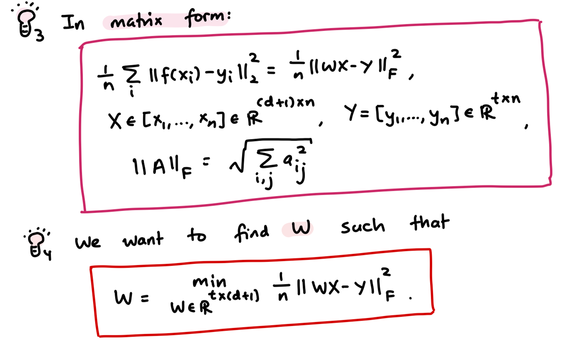
• Quick note on ==$\Vert A{\Vert }_F$== and the use of it in the above
  • a way to measure the “size” of a matrix that generalizes the notion of the Euclidean norm of a vector to matrices. It is defined as the square root of the sum of the squares of all the elements of the matrix.

Ok, so we have what we want to use to find our model weight $w$, how should we go about solving this linear regression. The above formulates what the objective function is that we are trying to minimize. To move forward, we need to start looking at how the model will take the mean squared error and learn from it. So, we have this loss function that is mean squared error, and we need to derive from a this, a value to adjust our model weight. To do this, we need to find the derivative of the loss function, and apply gradient descent. Before we can jump into this, we need a review on some of the concepts in calculus, which we will see now.

---

Calculus Detour

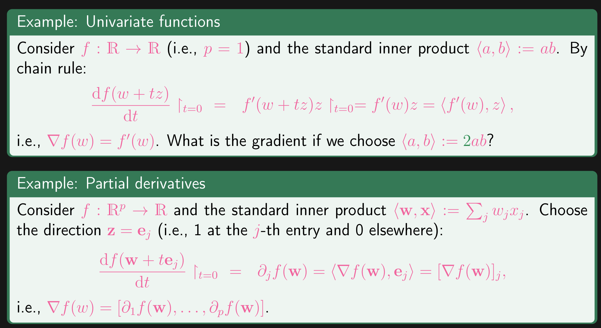
Let’s consider the function $f:{\mathbb{R}}^p\to \mathbb{R}$ be a smooth real-valued function. We fix an inner product, and define the gradient $\nabla f:{\mathbb{R}}^p\to \mathbb{R}$ as:

$\frac{df(w+tz)}{dt}{\upharpoonright }_{t=0}=⟨\nabla f(w),z⟩$

Something to note — The symbol $\upharpoonright$ is called the “restriction” symbol in mathematics, so in the above, we are restricting the expression or operation to the case where $t=0$

We will fix an inner-product, which just means to define some affine operation between the 2 values being dotted. Also, recall what the gradient represents: gradient of a function points in the direction of the greatest rate of increase of the function. To break down the above, we re-visit some multi-variable calculus knowledge.

→ Directional Derivative

In multivariable calculus, the directional derivative of a function $f(x,y)$ at a point $P$ in the direction of a vector $v$ measures the rate at which the function changes at $P$ as you move in the direction of $v$ It tells you how fast the function is changing at $P$ if you move in a specific direction. Mathematically, the directional derivative $D_{v}f(P)$ of $f$ at $P$ in the direction of $v$ is given by the dot product of the gradient of $f$ at $P$ and the unit vector in the direction of $v$:

$D_{v}f(P)=\nabla f(P)\cdot \hat{v}$

Where:

• $\nabla f(P)$ is the gradient (vector of partial derivatives)

• $\hat{v}$ is the unit vector in the direction of $v$

Let’s see a quick example. Consider the function $f(x,y)=x^2+y^2$. Graphically, it is:

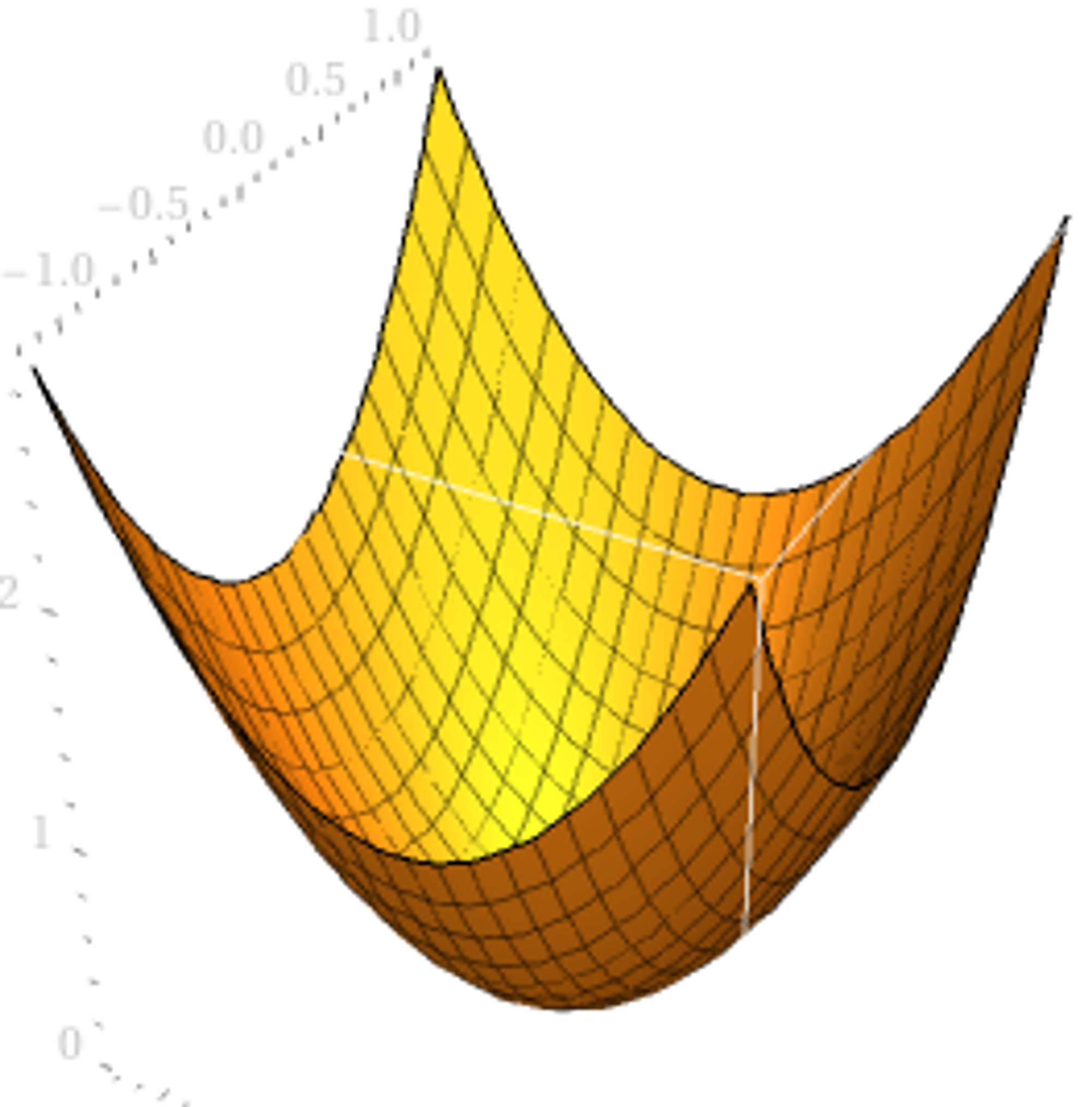
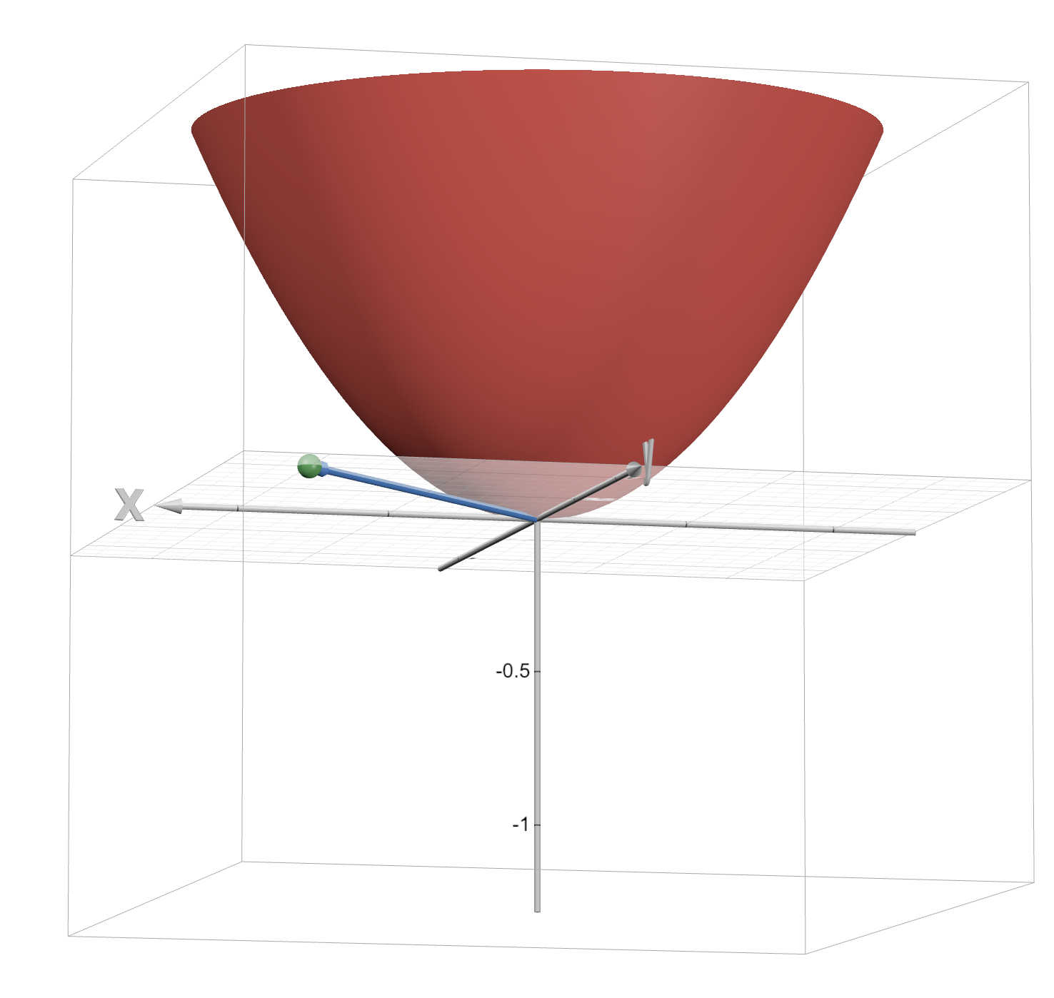
Let $P=(1,1)$ in the direction of the vector $v=(1,1)$. So, on the right, we see all 3 plotted.

1. Gradient of $f$:
   1. $\nabla f(x,y)=(2x,2y)$
2. Unit vector in the direction of $v$
   1. Normalize $v$ into a unit vector: $\hat{v}=\frac{v}{||v||}=(\frac{1}{\sqrt{2}},\frac{1}{\sqrt{2}})$
3. Compute the dot product:
   1. $\nabla f(1,1)\cdot (\frac{1}{\sqrt{2}},\frac{1}{\sqrt{2}})=(2x,2y)\cdot (\frac{1}{\sqrt{2}},\frac{1}{\sqrt{2}})=(2,2)\cdot (\frac{1}{\sqrt{2}},\frac{1}{\sqrt{2}})=2\sqrt{2}$

So, this means the directional derivative is $2\sqrt{2}$. So, it is now very obvious what we are trying to use this for: we will move the data point $P$ in the opposite direction of the gradient, as to move ourselves towards a local minima, minimizing mean squared error, and therefore improving the performance of the model.

Moving back to the Chapter 2- Linear Regression, we recognize that this is simply saying the rate of change in our regression function $f$, near the point $w$, along the curve $w+tz$ at $t=0$, is equal to the rate of change of $f$ at $w$ in the direction $z$. So, why is this important? This gradient is what we are looking for, and we obtain it through finding the derivative of the loss function. The following examples cover some of the calculus aspect of this:

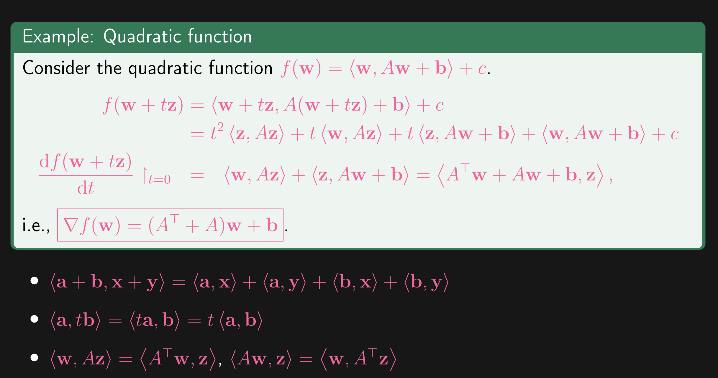
Small note on the quadratic function: This is a quadratic function for vector variables

• $⟨w,Aw+b⟩+c$
• $w^T(Aw+b)+c$
• $w^{T}Aw+w^{T}b+c$

This term resembles the 1D Vectors: $a{x}^2+bx+c$. So, $w^{T}Aw$ is the quadratic term, as all variables in $w$ are multiplied against each other, with some constants in $A$. Same applies for $w^{T}b$ and $c$

So, now we have looked the basics of calculus needed to compute the direction for learning. We move onto the next topics

---

Optimality Condition

Theorem: Fermat’s necessary condition for extremity
If
$w$ is a minimizer (or maximizer) of a differentiable function $f$ over an open set, then $f^{\prime }(w)=0$

A.K.A, we’re looking for local/global minimum for our loss function. We know have the tools to solve linear regression. So, we define the loss function:

$Loss(W)=\frac{1}{n}||WX-Y|{|}_F^2$

What does the $F$ subscript mean? The Frobenius norm $||A|{|}_F$ of a matrix $A$ is a measure of the “size” or “magnitude” of the matrix. It is defined as the square root of the sum of the absolute squares of its elements. It is the extension of the $||v|{|}_2$ seen for vectors.

Taking the derivative of this, with respect to $W$ and making the derivative equal 0:

${\nabla }_{w}Loss(W)=\frac{2}{n}(WX-Y)X^T=0$

So this is our model weight. Once we have solved for $W$ on the training set $X,Y$, we can predict on unseen data $X_{test}$: ${\hat{Y}}_{test}=W{X}_{test}$, where ${\hat{Y}}_{test}$ is the predictions our model makes on test data. The “test error” (if true labels were available):

$\text{test error}=\frac{1}{n_{test}}||y_{test}-{\hat{y}}_{test}|{|}_F^2$

The training error is:

$\text{training error}=\frac{1}{n}||Y-WX|{|}_F^2$

We will reduce the training error to reduce the test error.

---

Ill-Conditioning

Ill-conditioning in machine learning, particularly in the context of numerical optimization and linear algebra, refers to situations where a problem is sensitive to small changes in input.

---

Ridge Regression

What is ridge regression? Ridge regression is an extension of linear regression, and is particularly useful when we suspect the dataset has multicollinearity. What is this? We are now comfortable with the concept of regression, and have seen what simple linear regression is. This is very easy to imagine, i.e predicting housing prices from the crime rate in an area, for example. What about multiple predictor variables? That is, let’s consider multiple linear regression, where the model predicts the dependent variable using multiple independent variables.

This is good and all, until we consider the possibility of the IV’s have relationships between themselves and not being independent from each other, and this issue was mentioned in STAT231. multicollinearity refers to the above situation, where two or more predictor variables are highly correlated, causing problems in estimating the coefficients of the regression model, leading to unreliable and unstable estimates. To address this, we introduce a penalty for large coefficients. Let’s take a closer look at this.

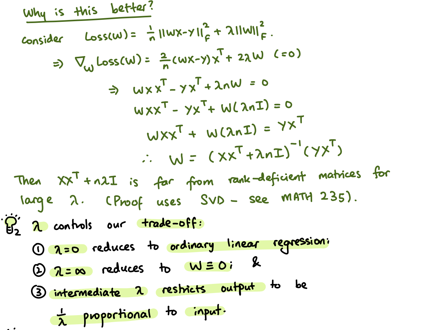
With Ridge Regression, our loss function becomes:

$Loss(W)=||XW-Y|{|}_2^2+\lambda ||W{|}_2^2$

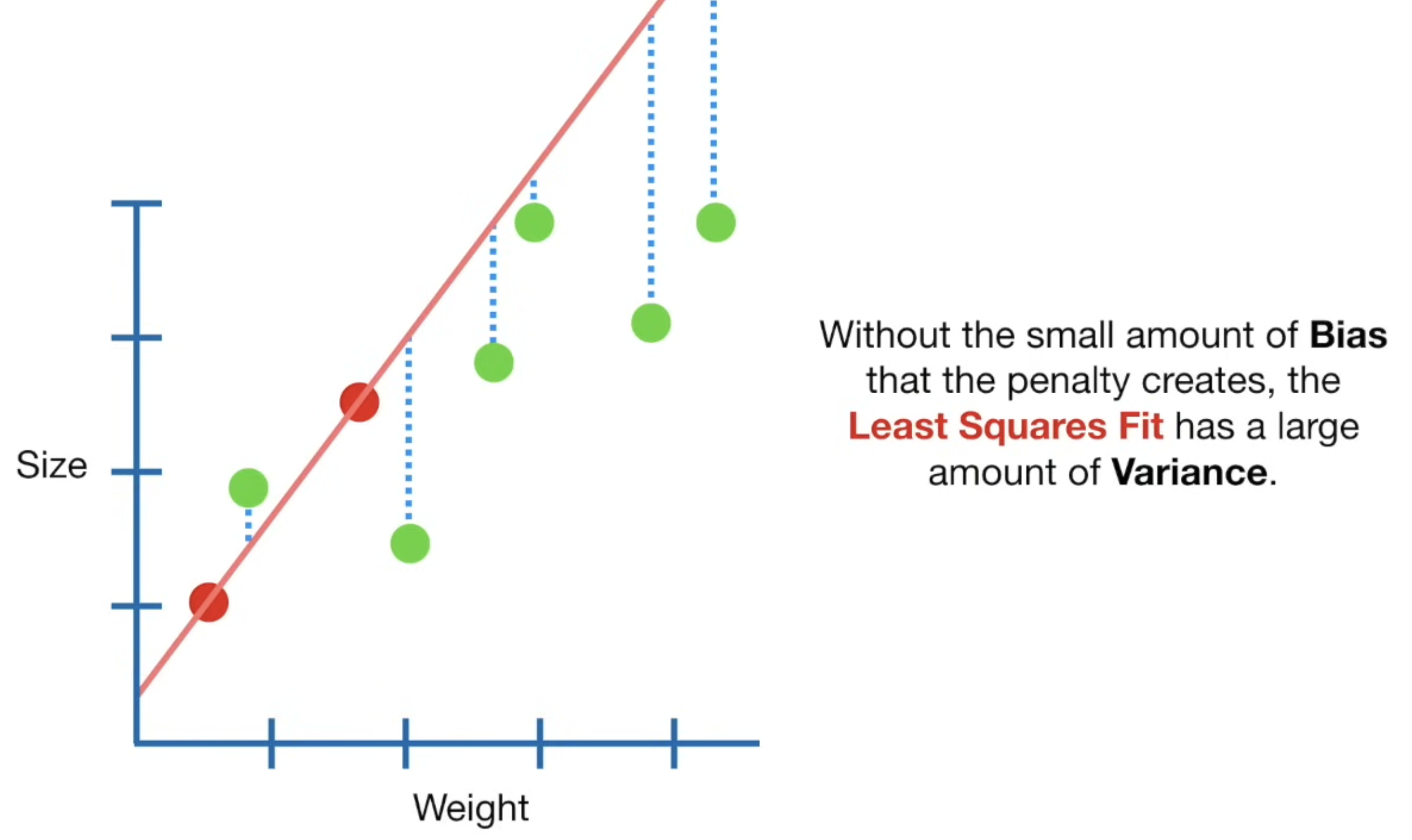
Where lambda is the penalty, a non-negative hyperparameter that controls the amount of regularization. The $\lambda ||W{|}_2^2$ term adds penalty for large coefficients, and scales with the value of $\lambda$. The choice of $\lambda$ is crucial. If $\lambda$ is too small, ridge regression behaves similarly to Ordinary Least Squares regression. If $\lambda$ is too large, the model may underfit the data by shrinking the coefficients too much. Cross-validation is commonly used to find an optimal $\lambda$, which we will see later on.

By shrinking the coefficients, it reduces the variance introduced by multicollinearity, leading to more stable and interpretable models. Here is a simple image demonstrating this:

So now, the problem boils down to finding the weight $w$, such that:

$w=\underset{W}{\min }[\frac{1}{n}||WX-Y|{|}_F^2+\lambda ||W|{|}_F^2$

To summarize this section, we’ll take an excerpt from other notes again:

⇒ Data Augmentation

To combat the issues of small datasets and the risks that come with that (e.g training on the same sample twice), much like CNN’s, we can introduce data augmentation. For ridge regression, we can augment the sample and corresponding label as so:

1. Augment $X$ with $\sqrt{n\lambda I_n}$: i.e $\tilde{X}=X\sqrt{n\lambda I_n}$
2. Augment $Y$ with zeroes: i.e $\tilde{Y}=(Y0)$

This is how we can achieve regularization.

⇒ Cross Validation

Know, just skip.