Lecture 10- Graph Algorithms 1

Graphs

A graph is a pair $G = (V, E)$
$V$ contains vertices and $E$ contains edges
- An edge $uv$ connects 2 distinct vertices $u, v$
We can have undirected graphs (no direction) and directed graphs (edges are arrows, and have direction)
- $(u, v) \neq = (v, u)$

Properties of Graphs

Number of vertices is $n = ∣ V ∣$ and number of edges is $m = ∣ E ∣ \leq n (n - 1)$ → note: $n (n - 1)$ is an instance of where each vertex is connected to every other vertex
- Note $m$ is in $O (n^{2})$ but not necessarily in $Ω (n^{2})$
- For undirected graphs, $m \leq \frac{n ( n - 1 )}{2}$
Indegree of a node $u$ , denoted $in d e g (u)$ , is the number of edges directed into $u$
Outdegree of a node, denoted $o u t d e g (u)$ , is the number of edges directed out from $u$
The neighbours of $u$ are the nodes $u$ points to
- also called the nodes adjacent to $u$ , denoted $a d j (u)$

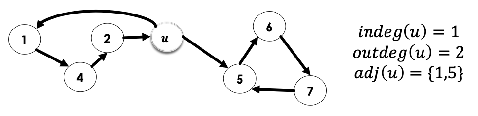
Data Structures for Graphs

There are 2 main representations we learn for graphs:

Adjacency Matrix
Adjacency List

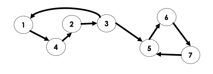
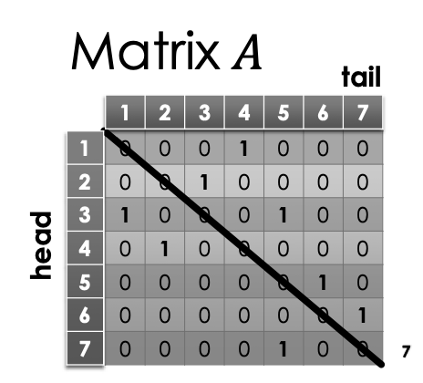
Adjacency Matrix Representation

$n$ x $n$ matrix $A = (a_{uv})$ , where rows and columns are indexed by $V$

$a_{uv} = 1$ if $(u, v)$ is an edge
$a_{uv} = 0$ if $(u, v)$ is a non-edge
Having a diagonal full of 0’s (so edges between the same vertex 1,1 or 2,2) means no self edges

This is for a directed graph. An undirected graph largely has the same matrix representation. However, we $(u, v)$ is the same as $(v, u)$ , then the matrix $A$ will be symmetric over the diagonal, in other words, $A = A^{T}$ transpose.

→ Implementing Adjacency Matrix

Suppose we are loading a graph from input. Assume the nodes have been labeled $0... n - 1$ and we are constructing a 2D boolean array → **bool adj[n][n]** → remember the first index is the head node and the second index is the tail node.
If the nodes in input are not labeled from $0... n - 1$ ? We can simple perform some pre-processing and rename them → probably through some hashmap
If needed, we can convert our 2D array into 1D array → adj[u][v] -> adj[u*n + v]

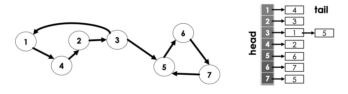
Adjacency List Representation

$n$ linked lists, one for each node
We write $aj d [u]$ to denote the list for node $u$
$a d j [u]$ contains the labels for nodes it has edges to. Below is an example:
- Note, does not neccessarily need to be a linked-list, array or any other similar data structure would also suffice
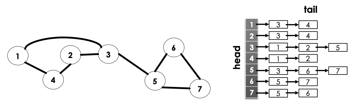
For undirected graphs, similar situation with the adjacency matrix → if 2 points to 3 then 3 also points to 2.

→ Implementing Adjacency Lists

Suppose we are loading a graph in from input.

Assume nodes are labeled from $0... n - 1$
Construct an array (or vector, anything along these lines) would work =

BFS (Breadth First Search)

Consider the following code:

def BreadthFirstSearch(V[1...n], adj[1....n], s):
	pred[1...n] = [null, null, null, ..., null]
	dist[1...n] = [infty, infty, infty, ..., infty]
	colour[1...n] = [white, white, ..., white]
	q = new queue
 
	colour[s] = gray
	dist[s] = 0
	q.enqueue(s)
 
	while q is not empty:
		u = q.dequeue()
		for v in adj[u]:
			if colour[v] = white:
				pred[v] = u
				colour[v] = gray 
				dist[v] = dist[u] + 1
				q.enqueue(v)
		colour[u] = black
 
return colour, pred, dist

For this, we assume that adj is in the adjacency list representation
Undiscovered nodes are white ,discovered nodes are gray, and finished nodes are black
We process adjacent edges, hence why we push all adjacent edges onto the queue
S will be our start node
We maintain a pred which is a predecessor array. This will be set when we discover a node, the predecessor will be the node that we came from to discover a particular node. Starts as null as before we have even discovered the node, we do not know the predecessor
dist is the distance in the number of hops (number of edges traversed) to get from start node to each node. We initialize this to $\infty$ as the algorithm will shrink/look for min.
We make the colour of the starting node gray, as are on it, and we make it’s distance in dist to be 0, as we are starting from that node. Then, we add it to the queue. In BFS we always maintain a queue of the next to be processed (adjcaent nodes), nodes that are still interested in visiting and processing.
So, we first pop the first element from the queue, and then add all of it’s adjacent nodes to the queue if we have not visited them before. We can accomplish this with a set, or in this case, a colour array.
- If white (unvisited), we make the predecessor of that node the current node we are on (u), make the colour of it gray, and assign it a distance (current distance + edge weight, 1 in this case). We then mark our node (u) black to indicate it is visited.
Then, we add it to the queue and iterate. We continue this algorithm until the queue is empty → no more nodes to visit

We can start this algorithm at any node (while in bst, we would start this on the root node). So, what is the time complexity of this algorithm?

Constructing the first 3 arrays is a $O (n)$ time operation.
Creating the queue and queue operations are all $O (1)$ constant time
The while loop is $O (n)$ as there are at most n nodes we can possibly visit and add to the queue. In inner for loop is a $O (∣ a d j [u] ∣)$ operation as the for loop iterates that many times (bounded by n as each node is at most n-1 adjacent nodes).
All the operations inside of the inner if statement is constant $O (1)$ time

So, overall, this runtime is dominated by the $O (n)$ iterations x $O (∣ a d j [u] ∣) \leq O (n)$ iterations → $O (n^{2})$ runtime. While this is important to know, we ideally would like to obtain a $Θ$ notation bound for this algorithm. So, how do we do this? First of all, we need to do a smarter analysis of the run time of the for loop in the above. Consider this, instead of considering each loop independently, consider them together and the total work they do together.

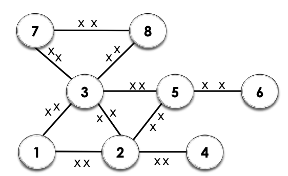
So, consider the graph above. Notice that throughout the 2 loops, we visit every node and do work on every edge. But, as we visit each neighbour for each node, as expected, we will have done something to each edge twice (once when we visit the first end node, and the second when we visit the other end node). So, this means we will do $O (m)$ work over all edges. For each node, if we iterate over every neighbour, we will see edge twice. So, there are $O (n + m)$ work total if we iterate over every node and for each node, for all neighbours. So:

Total contribution of the inner loop: $O (m)$ over all iterations of the outer loop, and in outer loop, we do $O (n)$ work.
So, total run time is $O (m + n)$

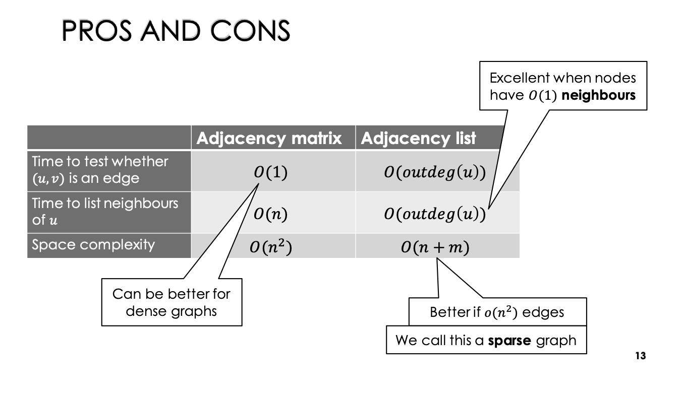
→ So, this is us doing this algorithm with a adjacency list, what if we instead used an adjacency matrix? The analysis is mostly similar to what we’ve seen above, but now, as we do not have a list to adjacent nodes, it takes $O (n)$ time to determine which nodes are adjacent to u. This cost is paid for each u, resulting in a total runtime of $O (n^{2})$ . Something interesting about this algorithm is pred array. The way that it is constructed in a connected graph, the pred array induces a tree.

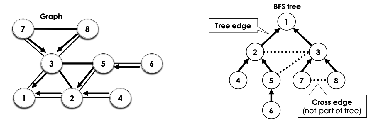
This is because we have made every node’s predecessor in the pred array be the node we came from in the BFS → Every node started from the start node, and so, we obtain this tree structure. In the diagram above, in the left diagram, the arrows are called tree edges as they are edges in the BFS tree. Edges in the graph (such as the one between 7 and 8) are called cross-edges and they are not in pred as they are not apart of the BFS tree.

BFS: Proof of Optimal Distances

BFS actually computes the shortest path from the start node s to any other node u in the graph → This information is stored in the distance array So, we want to prove this, and we will use the BFS tree to do this.

→ Distance in Graph $G$ and BFS tree $T$

Denote $d_{G} (v)$ as the (optimal or shortest) distance between s and v in graph $G$
Denote $d_{T} (v)$ as the distance between s and v in the BFS tree $T$
Recall that dist[v] is a value set by the BFS Algorithm for every node of the graph

High-level Proof Idea:

The idea is, at the end of the BFS, dist[v] = $d_{G} (v)$ for all $v$ . We can split this into 2 parts:

Claim 1: dist[v] = $d_{T} (v)$
Claim 2: $d_{T} (v)$ = $d_{G} (v)$

→ Sketch of Claim 1

To prove this, we first make a key observation in the BFS algorithm: whenever we set dist[v] = dist[u] + 1, u is the parent of v in the BFS tree. So, we could make an inductive proof to show dist[v] = $d_{T} (v)$

e.g. by strong induction, on the nodes in the order their dist values are set
Say you have a sequence of nodes in the order their distance values are set. We assume that up to the $i$ th node that has it’s distance set in the BFS, all of those distances are exactly equal to $d_{T} (v)$ . Then, prove the $i + 1$ th node. Then, since the previous nodes have dist values exactly equal to $d_{T} (v)$ , we can use this to finish the proof.

→ Sketch of Claim 2

We prove this through proving $\forall v, d_{G} (v) \leq d_{T} (v)$ as well as $\forall v, d_{G} (v) \geq d_{T} (v)$ . In proving both directions, we will have proven claim 2.

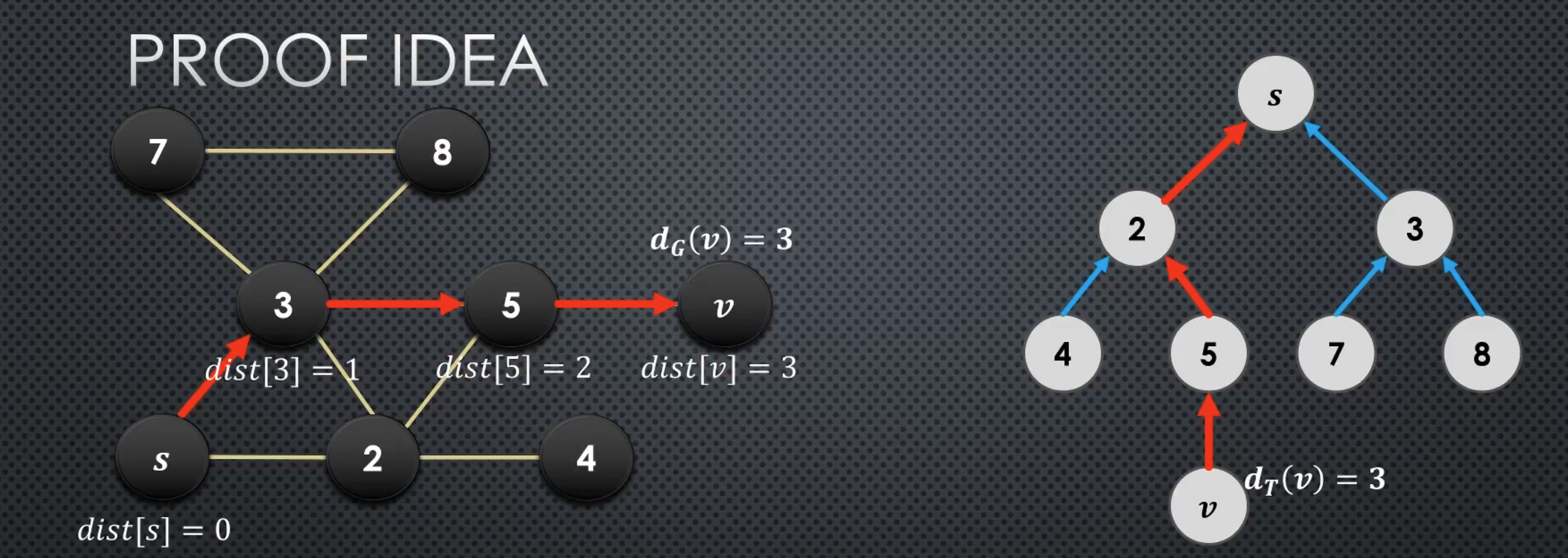
→ Direction
- We know there is a unique path that goes $v$ → … → $s$ in $T$ (from the node v to th start (root) node s)
- $T$ is a subgraph of $G$ (recall we saw that all the arrows in the tree $T$ are edges in $G$ , along with the cross edges
- So, that same path $v$ → … → $s$ also exists in $G$ (technically reversed, but same thing)
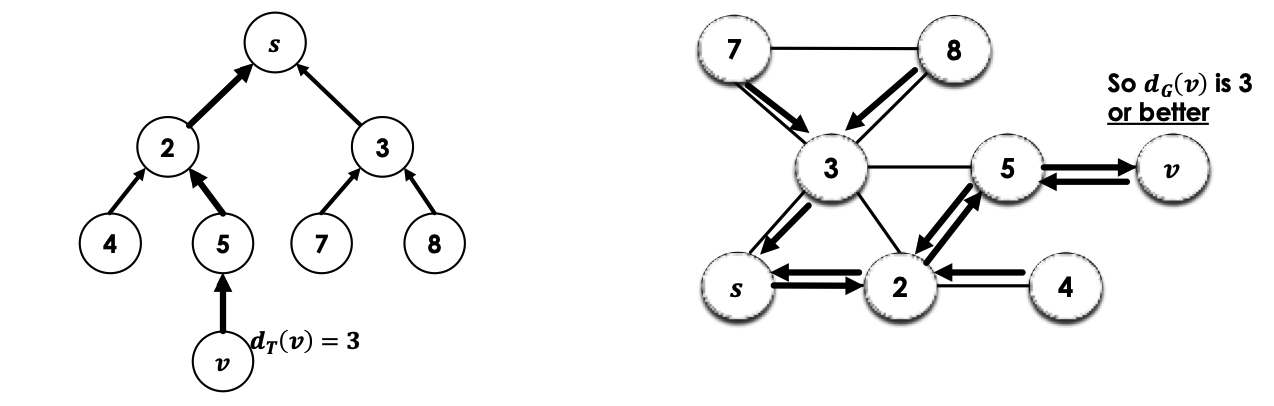
← Direction
- We partition the tree $T$ into levels → $V_{i} = {v : d_{T} (v) = i}$ by distance from the root node s
- We make the the “helper” claim that: there is no “forward” edge in $G$ that “skips” a level from $V_{i}$ to $V_{j}, j \geq i + 2$ .
  - Suppose for the sake of contradiction, there is an edge that goes “skips” levels from $V_{i}$ to $V_{j}$ , for example, from $V_{0}$ to $V_{2}$ . What are the consequences? To understand this well, it is beneficial to look at a diagram of that edge in $G$ .
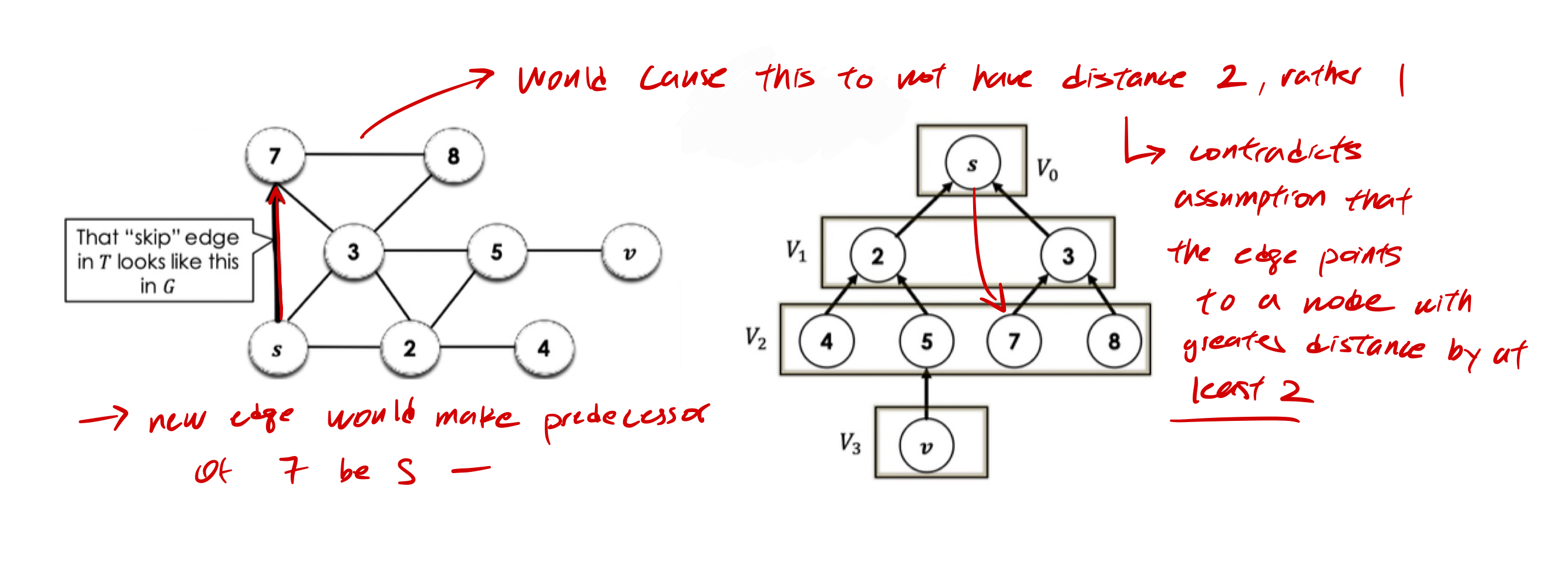
- So, we’ve just argued that there is no “forward” edges in $G$ that “skips” a level in $T$ from $V_{i}$ to $V_{j}, j \geq 2$
- Since no edge in $G$ “skip” a level in $T$ , we know at least one edge in $G$ is needed to traverse each level between $s \in V_{0}$ and $v \in V_{d_{T} (v)}$
- There are $d_{T} (v)$ such levels, so $d_{G} (v) \geq d_{T} (v)$

→ BFS Tree Properties

A interesting fact is that there are also no “back” edges in undirected graphs that “skip” a level going up the BFS tree.

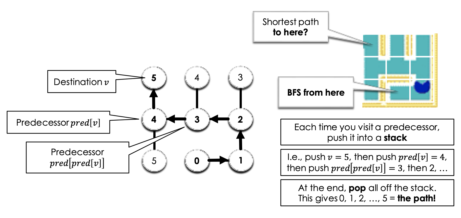
Application: Finding Shortest Paths

So, how do we actually output the path from s to v with minimum distance. The algorithm for this is actually fairly similar to extracting an answer from a DP array! We work backwards, starting from the node v and move backwards with the predecessors array. This will print the path in reverse, to resolve this, we can push every node we visit through this traversal into a stack. Then at the end, we can pop everything and form an array of the proper order.

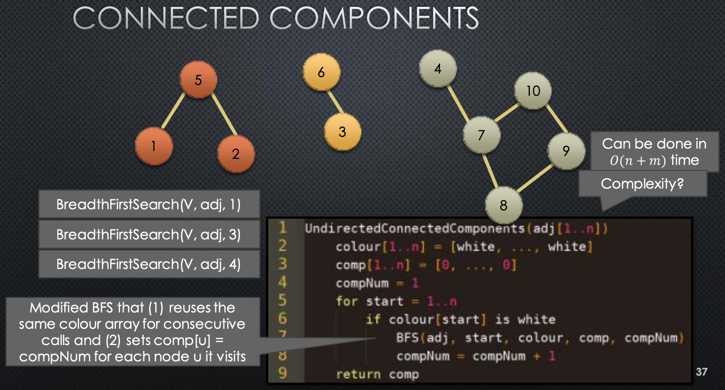
Application: Undirected Connected Components

→ Example: undirected graph with three components

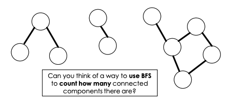
Say for this graph $G$ , we want to know how many components there are. So, how can we do this → How can we use BFS to compute this?

We have nodes labels from $1$ … $n$
We will perform a bfs on node 1, which will visit some subet of nodes → marking them as visited → once this bfs has finished, we have found one component
We then look at te next nodes in our input → 2,3…. $n - 1$ until we find a node that has not been visited
We then call bfs on that node

After this, we will have found the number of components in our graph.

💻 Allan Yin's Blog

Explorer