Chapter 5- Fully Connected Neural Network

Consider the XOR problem on some example data:

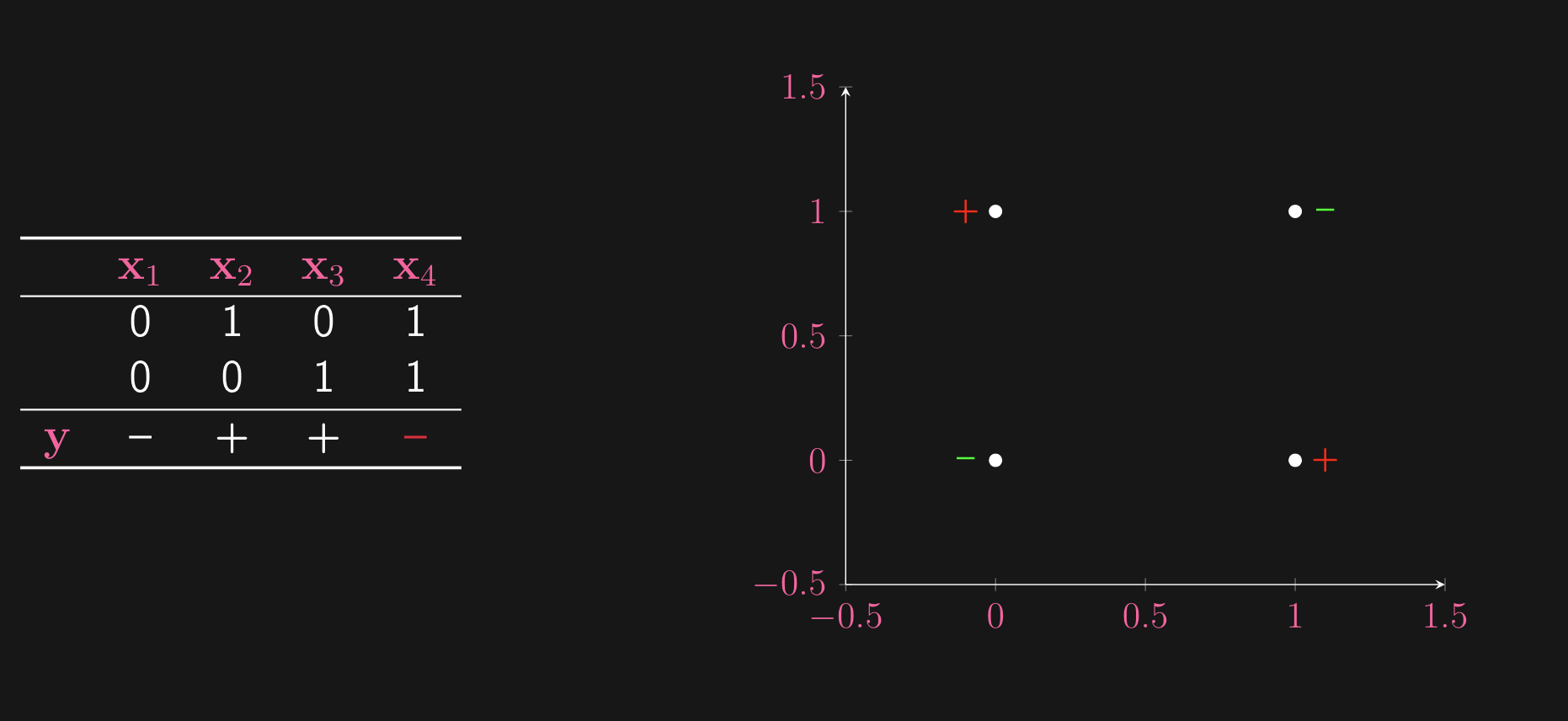
What do we see? This is no separating hyperplane for this dataset. So, we cannot fit a hyperplane to this data. We can consider 2 solutions:

1. Fix input representation but use a richer model (e.g ellipsoid)
2. Fix hyperplane as classifier but use a richer input representation

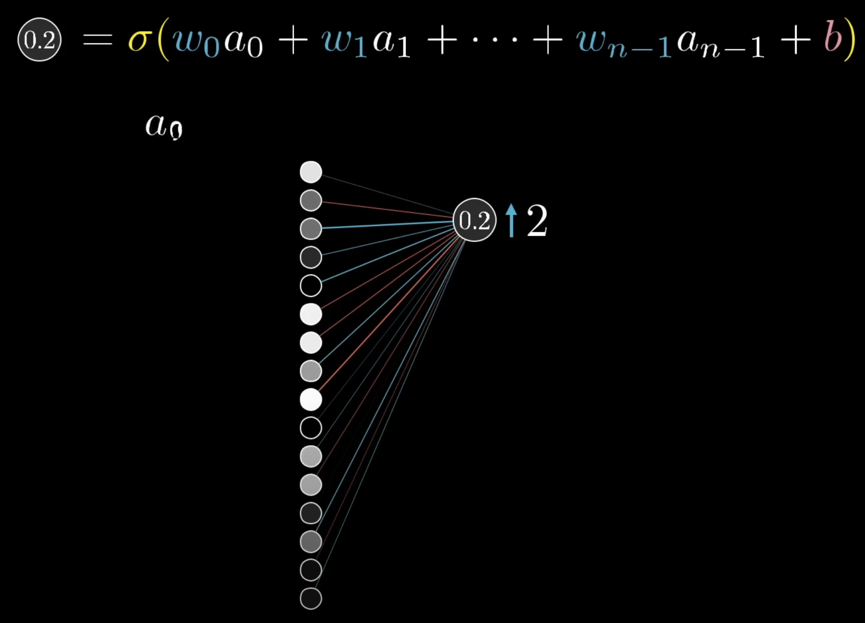
These 2 are the same, through a reproducing kernel. What a neural network does is it learns the feature map simultaneously with the hyperplane (hence you visually get the idea of the entire Hilbert space rotating and shifting). Now, recall that our perceptron model took on the following form:

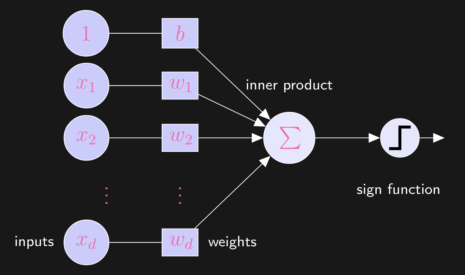
Where we take the inner product of our data point $x\in {\mathbb{R}}^d$ and the weight vector $w$, and pass the result to the sign function, which maps this result to one of the output options (predicting a value, or labeling it as + or - for binary classification, etc.) Now, we can add more layers to the perceptron, forming a multi-layer perceptron:

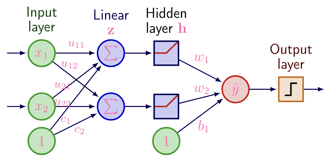
• 1st linear transformation: $z=Ux+c,U\in {\mathbb{R}}^{2x2},c\in {\mathbb{R}}^2$
• Element-wise nonlinear activation function (to help learn non-linear relationships in the data); makes all the difference!
• 2nd linear transformation: $\hat{y}=⟨h,w⟩+b$

Now, you can probably see the inklings of a neural network. We have weight matrix $U$ and we multiply it by input vector $x$, add the bias, and this is the output of the first layer. Then, we take this output, apply some non-linear activation function, and then feed it to a final output layer, where the linear mapping between this result and prediction, is learned. The above case is when there is only value to be predicted, so in the basic perceptron binary classification we saw, this is $+1$ or $-1$. Of course, we’re not always going to be doing classification tasks, and so, a more general diagram of a standard dense, fully-connected neural network:

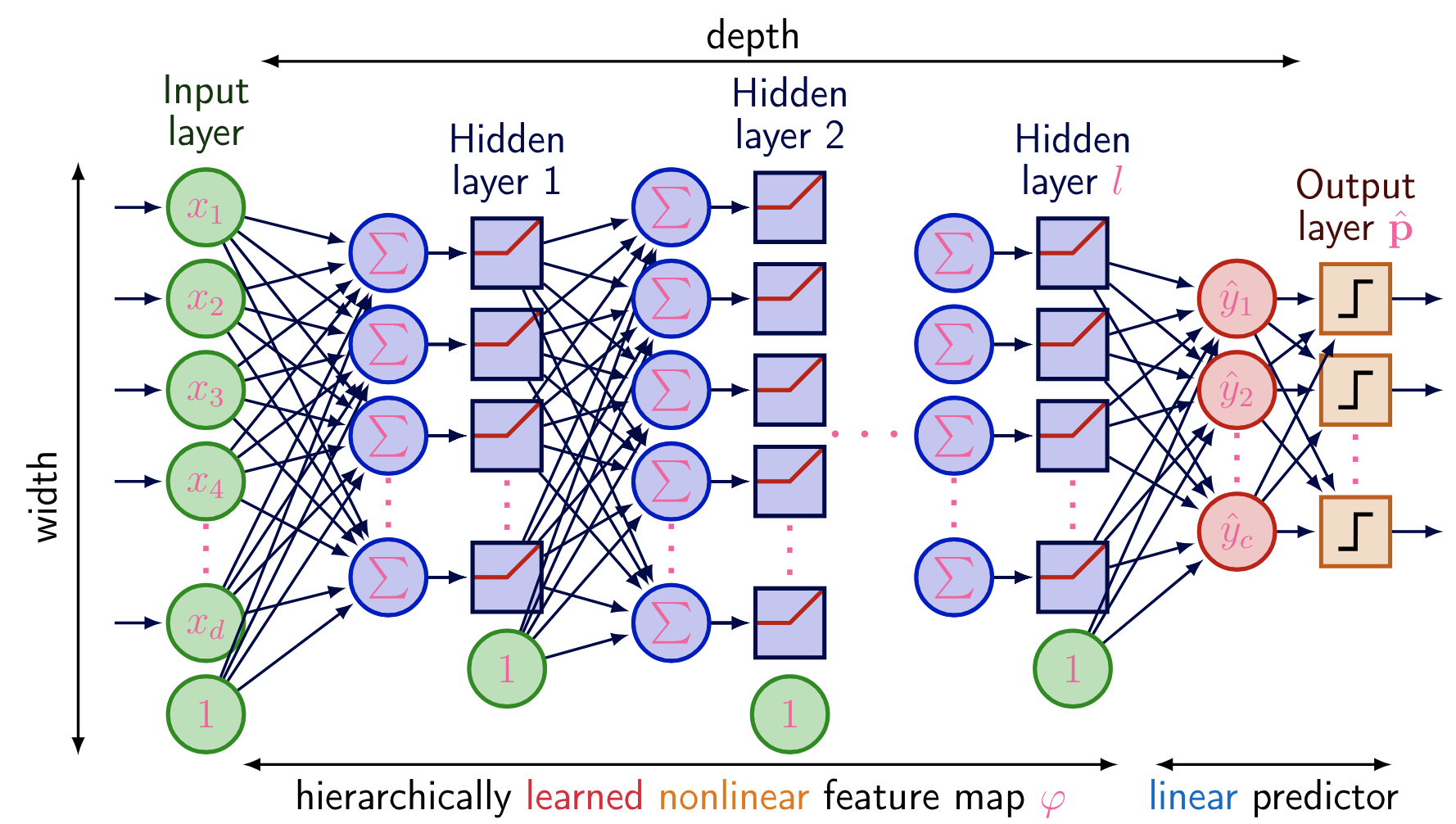
A couple things to note about our neural network:

• In the above, each layer has its own matrix weight $W$, where each neuron has its own vector weight. When $x_i$ has arc to one of the neurons, we are taking the inner product of one of the column vectors with the input vector. For a layer with $n$ neurons and an input vector of size $m$, the weight matrix $W$ has dimensions $m$ x $n$.
  • This is why the computation is $Wx$, this matrix multiplication is equivalent to the above
  • This will be important later on, when we consider the above as a Directed Acyclic Graph
  • Can also think of the values in each of these column vectors to be the arc costs
  • 
• We can have an arbitrary number of layers, and continue to increase our depth to create deep neural networks. However, keep in mind, the deeper the model, the more powerful it becomes, and the easier it is for the model to overfit on the training data, a critical issue with deep neural networks. As usual, we almost always will end off our NN with some dense linear layer, to map the results of the model with prediction labels.
• The input are now tensors, no longer simple vectors, this is especially the case when we mention batch training

Let’s see an example of iterating through a MLP (Multi-layer Perceptron) model, over test data set (since we haven’t yet seen how to do backtracking)

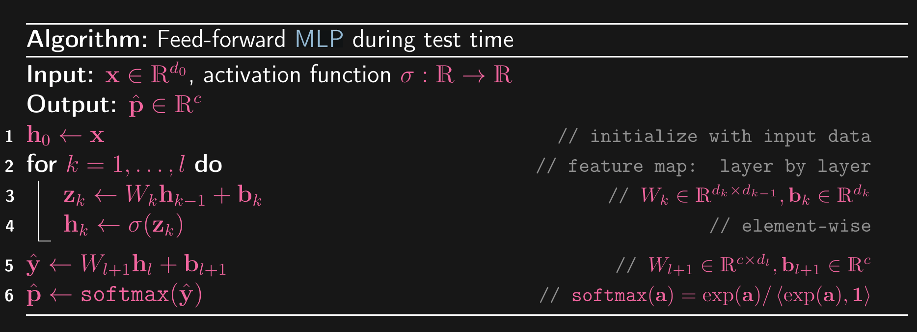
Now the above is very simple. We have $l$ layers in our model, hence, we iterate from $k=1$ until $k=l$. So, each layer has weight matrix $W_k$, and then we go through the same motions: (1) Multiply weight by the output $h$ of the previous layer (which in the first iteration, is just the input data), and add on the bias term. Then, we pass this through a non-linear element-wise activation function, and assign this to the output of this layer.

• At the very end of this loop, we take the output of these layer, and run it through one final dense linear layer, before passing it to final activation function Softmax, which is commonly used as the last activation function of an NN to normalize the output of a network to a probability distribution over predicted output classes.

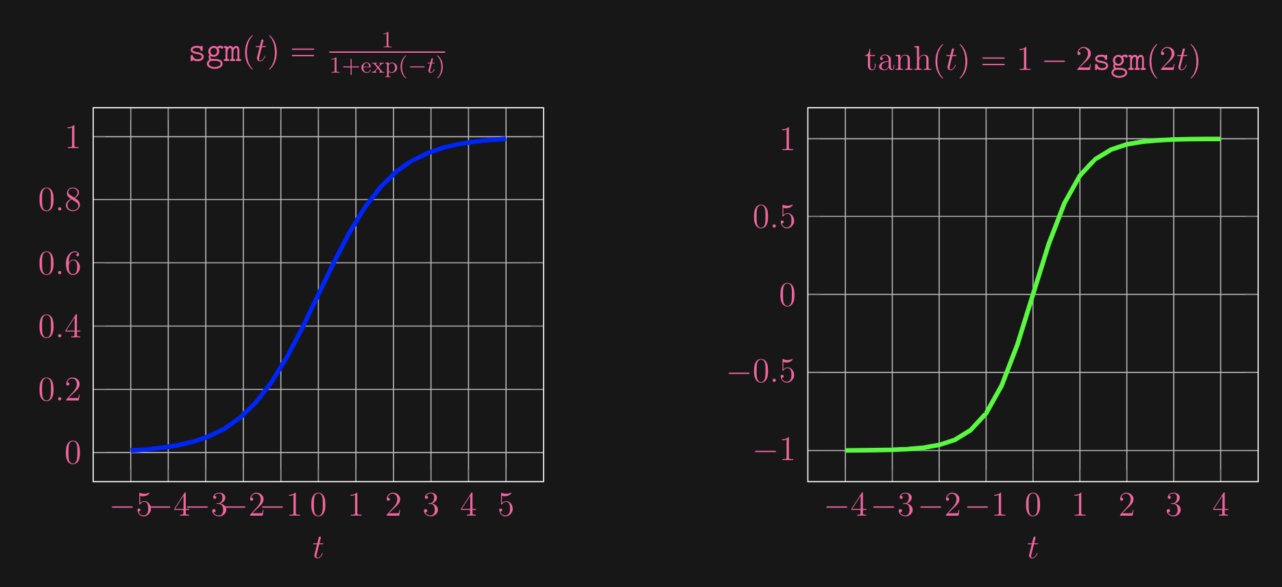
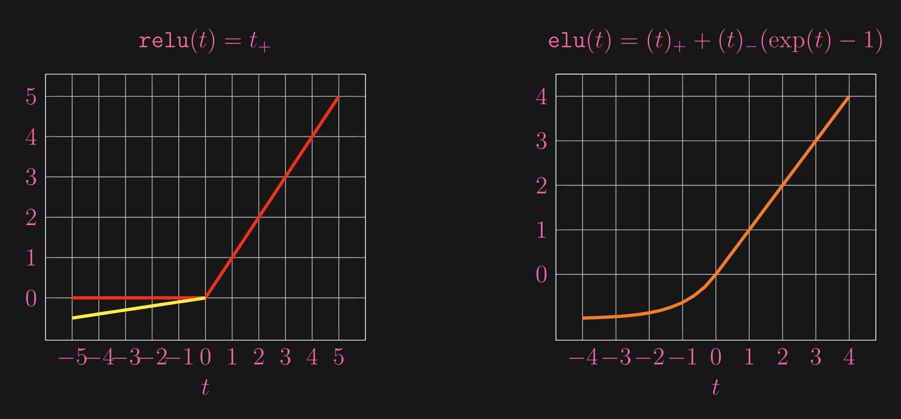
So, thats clear, here’s just a quick look at what some example activation functions look like: Now, let’s take a look at what happens during training for NN/MLP, as there is where the magic happens!

→ Training For the NN, we need a loss function. We define this function $l$ and we use it to measure the difference between prediction $\hat{p}$ and truth $y$. This can be through things like squared loss or through something like log loss. So, how does the model learn? The core concept is in backpopogation and gradient descent.

$$\underset{w}{\min }\frac{1}{n}\sum _{i=1}^n[\ell \circ f](x_i,y_i;w)$$ $$w\leftarrow w-\eta \cdot \frac{1}{n}\sum _{i=1}^n\nabla [\ell \circ f](x_i,y_i;w)$$

This is the loss function we are interested in. In the training phase of a Multi-Layer Perceptron (MLP) or any neural network, the goal is to find the set of weights that minimizes the average loss over all training data, hence, we are looking for mine $w$ that is average over ALL data points, where we are taking loss function $l$ of the model function $f$.

Then, to learn, we need to minimize average loss, optimization algorithms such as Gradient Descent are used. The basic idea is to iteratively adjust the weights www in the direction that reduces the loss. This is done by computing the gradient of the loss function with respect to the weights and updating the weights as follows:

$$w_{t+1}\leftarrow w_t-\eta \nabla g(w_t)$$

Visually, imagine this as:

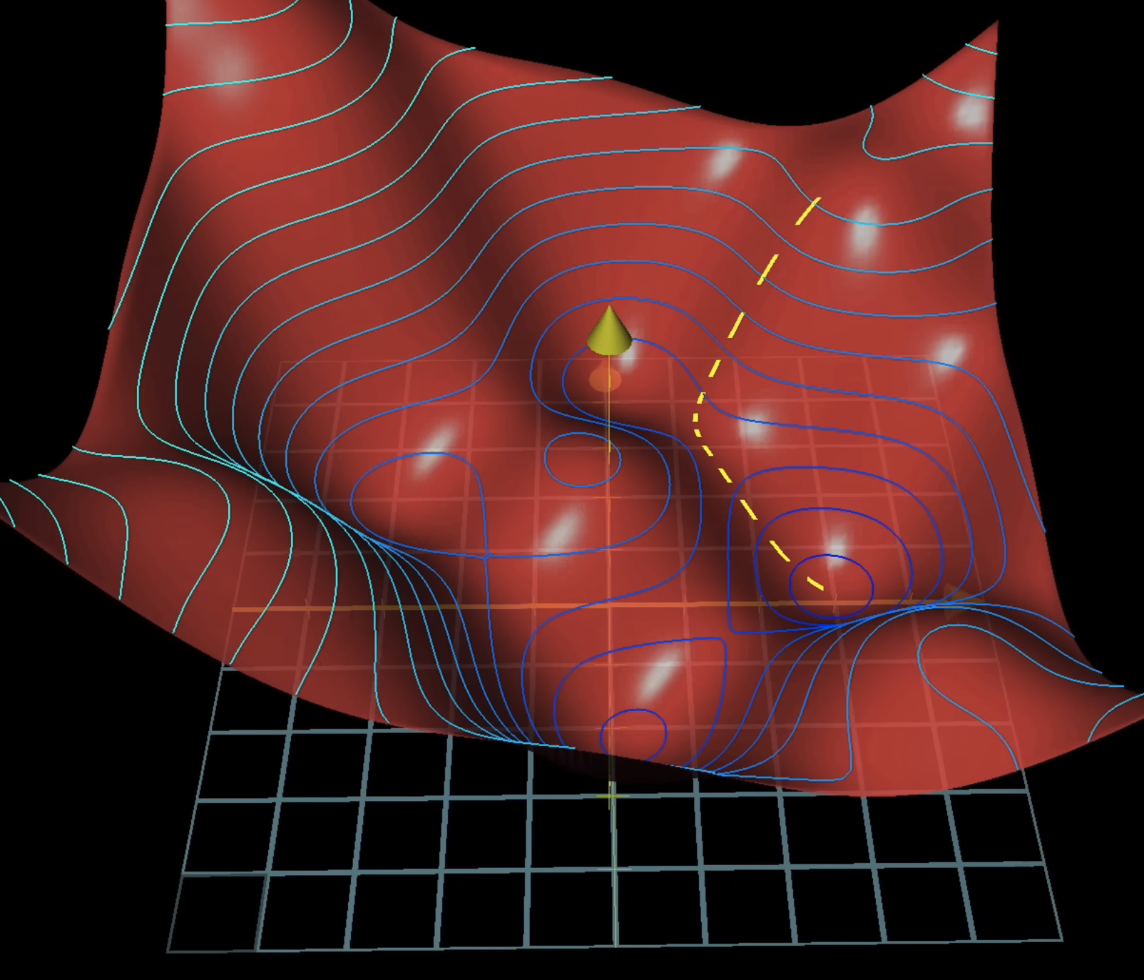
There are 2 things we should mention here: (1) Learning rate and (2) Batch size.

Learning Rate

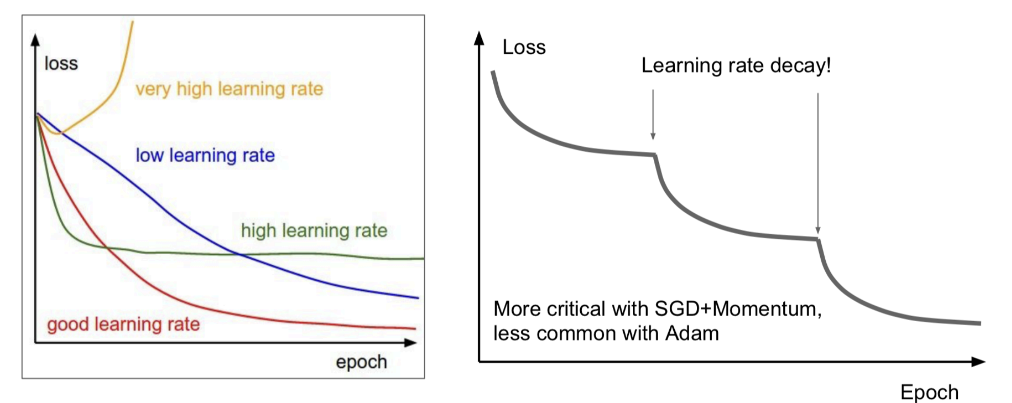
where $\eta$ is the learning rate, which controls the size of the weight updates, the step size if you will, and ${\nabla }_{w}L$ is the gradient of the loss with respect to the weights. This step size is very important. Why?

• Consider if the learning rate is too high, then, we run the risk of missing local/global minima of the loss function (imagine this graphed in higher-dimension)
• If the learning rate is too low, then, we will take too long to find minima, or become stuck

Batch Size

Each iteration will required a full pass over the entire training set! So, to adjust the weights ONCE, we need to iterate over the ENTIRE dataset. This, while theoretically would provide the best learning, is incredibly expensive. A middle-ground for this is train in batches, so we run the batch of data, take average loss, and update the weights from that. We call this mini-batch , where we take some random set of data $B\subseteq \{1,...,n\}$ suffices:

$$w\leftarrow w-\eta \cdot \frac{1}{|B|}\sum _{i\in B}\nabla [\ell \circ f](x_i,y_i;w)$$

Moving forward, for the sake of simplicity, we’ll define

$$g(w_t)=\frac{1}{|B|}\sum _{i\in B}\nabla [\ell \circ f](x_i,y_i;w)$$

The average gradient over a mini-batch.

Momentum

→ Gradient Descent Basics Momentum is an optimization technique used to accelerate the convergence of gradient descent by adding a fraction of the previous update to the current update. It is designed to help gradient descent algorithms navigate the optimization landscape more effectively, especially in scenarios where the gradients oscillate or progress slowly.

→ Standard Momentum The standard one: $w_{t+1}\leftarrow w_t-\eta \nabla g(w_t)$. Now, how would this change with momentum. Consider:

$$\begin{array}{rl}{w}_{t+1}& =\underset{\text{gradient step}}{\underbrace{w_t-{\eta }_t\nabla g(w_t)}}+\underset{\text{momentum}}{\underbrace{{\beta }_t(w_t-w_{t-1})}}=\underset{\text{extrapolation}}{\underbrace{(1+{\beta }_t)w_t-{\beta }_t{w}_{t-1}}}-{\eta }_t\nabla g(w_t)\end{array}$$

Now, we look for a better way to represent momentum, we define variable $\tilde{v}$ represent a form of momentum or velocity in the optimization process. In the above, ${\beta }_t$ to be the momentum coefficient for the momentum term. Notice that momentum incorporates the previous weight as well. We define intermediate $\tilde{v}$:

$${\tilde{v}}_{t+1}=\beta {\tilde{v}}_t+{\eta }_t\nabla g(w_t),\text{where we get }{\tilde{v}}_{t+1}=w_t-w_{t+1}$$

We say intermediate velocity because it represents a temporary calculation that combines the effects of the current gradient and momentum before making the final update to the weights. Notice that this equation incorporates the previous velocity. Then, we can interpret the momentum as gradient averaging:

$$\begin{array}{rl}{v}_{t+1}& =\frac{{\alpha }_{t-1}}{{\alpha }_t}{\beta }_t{v}_t+\frac{{\eta }_t}{{\alpha }_t}\nabla g(w_t),\text{where }{\alpha }_t{v}_{t+1}=w_t-w_{t+1}\\ & =\underset{\text{gradient averaging}}{\underbrace{(1-{\gamma }_t)v_t+{\gamma }_t\nabla g(w_t)}},\underset{\text{gradient update}}{\underbrace{w_{t+1}=w_t-{\alpha }_t{v}_{t+1}}},\\ \text{where }{\alpha }_t& ={\alpha }_{t-1}{\beta }_t+{\eta }_t\text{ and }{\gamma }_t:=\frac{{\eta }_t}{{\alpha }_t}\in [0,1].\end{array}$$

Now, a couple things to note about this:

• This is essentially a weighted average, note how we are multiplying first term by $\frac{{\alpha }_{t-1}}{{\alpha }_t}$ and the second term by $\frac{1}{{\alpha }_t}$, and then adding together (comparing this to intermediate velocity).
• Then, after grouping like terms, the gradient averaging becomes clear:
  • Now that we have $v_{t+1}=(1-{\gamma }_t)v_t+{\gamma }_t\nabla g(w_t)$, then we can rearrange to obtain: ${\gamma }_t\nabla g(w_t)=v_{t+1}-(1-{\gamma }_t)v_t$. So, substituting this back into our gradient step, we can see how the new gradient update was derived: $w_{t+1}=w_t-{\alpha }_t{v}_{t+1}$.

So, what does this mean? We interpret this as the velocity is a weighted average of old velocity + some multiple of the gradient, where we usually choose $\gamma <1$. For example, say we make $\gamma =0.9$, this would mean we define the current velocity to be 90% of old velocity + 10% of the new gradient.

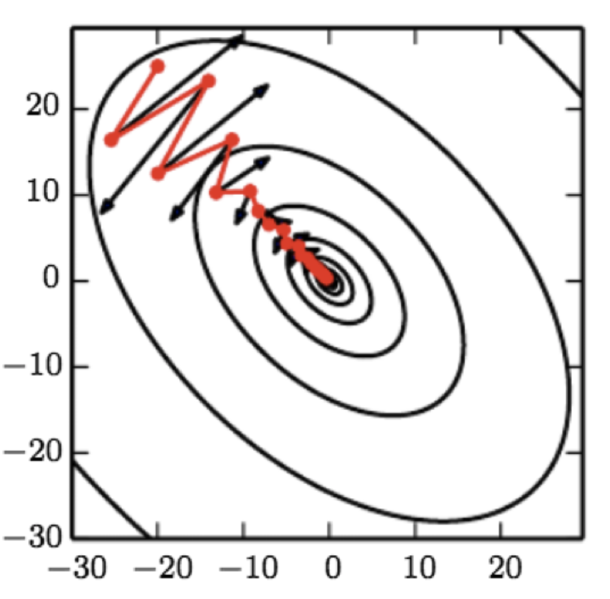
Look at this diagram, this illustrates why we need momentum. Without momentum, gradient updates would take the black line. With momentum, give more weight to the trajectory of the direction.

→ Nesterov Momentum Another interesting concept is Nesterov momentum, which is sometimes also called Nesterov Accelerated Gradient. This is very similar to the first velocity we derived above:

$$z_{t+1}=w_{t+1}+{\beta }_t(w_{t+1}-w_t)$$ $$\begin{array}{rl}{v}_{t+1}& =\frac{{\alpha }_{t-1}}{{\alpha }_t}{\beta }_t{v}_t+\frac{{\eta }_t}{{\alpha }_t}\nabla g(z_t),\text{where }{\alpha }_t{v}_{t+1}=w_t-w_{t+1}\\ & =\underset{\text{gradient averaging}}{\underbrace{(1-{\gamma }_t)v_t+{\gamma }_t\nabla g(z_t)}},\underset{\text{gradient update}}{\underbrace{w_{t+1}=w_t-{\alpha }_t{v}_{t+1}}},\\ \text{where }{\alpha }_t& ={\alpha }_{t-1}{\beta }_t+{\eta }_t,z_t=w_t-{\beta }_{t-1}{\alpha }_{t-1}{v}_t=w_t-{\alpha }_t(1-{\gamma }_t)v_t,\text{ and }{\gamma }_t:=\frac{{\eta }_t}{{\alpha }_t}\in [0,1].\end{array}$$

So, structurally, this is very similar to the above derivation for velocity. The more important one is the first momentum definition.

→ Optimizers What are optimizers? SGD is one of them, and these are the methods in which the model “learns”, or updates its weights. They define specific strategies for how the model’s parameters (weights) should be adjusted during training to minimize the loss function. Each optimizer implements a different algorithmic approach to weight updates, aiming to improve convergence speed and overall model performance. Here a couple of other commonly used ones, with each being favoured for different tasks like classification or regression. Let’s briefly look at 3 notable ones: Adagrad, RMSprop, and Adam:

First off, all 3 follow very similar skeleton:

$$w_{t+1}=w_t-\frac{{\eta }_t}{\sqrt{s_t+ϵ}}\odot v_t$$

→ Adagrad (Adaptive Gradient Algorithm):

$$\begin{array}{rl}{s}_t& =s_{t-1}+\nabla g({\mathbf{w}}_t)\odot \nabla g({\mathbf{w}}_t)\\ v_t& =\nabla g({\mathbf{w}}_t)\end{array}$$

• This method adapts the learning rate for each parameter based on historical sum of squared gradients (as seen above)
• Use Case: Suitable for sparse data and scenarios where the importance of features changes over time.

→ RMSprop (Root Mean Square Propagation):

$$\begin{array}{rl}{s}_t& =(1-{\lambda }_t)s_{t-1}+{\lambda }_t\nabla g({\mathbf{w}}_t)\odot \nabla g({\mathbf{w}}_t)\\ v_t& =\nabla g({\mathbf{w}}_t)\end{array}$$

• Modifies Adagrad by maintaining a moving average of the squared gradients to avoid decreasing the learning rate too much.
• Use Case: Personally, I’ve used this a lot when building personal models. Effective for non-stationary objectives and works well in practice for a variety of neural network architectures.

→ Adam (Adaptive Moment Estimation):

$$\begin{array}{rl}{s}_t& =(1-{\lambda }_t)s_{t-1}+{\lambda }_t\nabla g({\mathbf{w}}_t)\odot \nabla g({\mathbf{w}}_t)\\ v_t& =(1-{\gamma }_t)v_{t-1}+{\gamma }_t\nabla g({\mathbf{w}}_t)\end{array}$$

• Combines the ideas of RMSprop and momentum by maintaining both an exponentially decaying average of past squared gradients and past gradients.
• Use Case: Widely used due to its adaptive learning rates and momentum properties, making it suitable for a wide range of problems.

Computational Graph

This is just if we were to imagine the neural network as some acyclic digraph $D=(N,A)$, where $N$ is the set of nodes and $A$ is the set of arcs. We group the nodes into 3 categories:

$$\underset{\text{input}}{\underbrace{v_1,\dots ,v_d}}\underset{\text{intermediate variables}}{\underbrace{v_{d+1},\dots ,v_{d+k}}}\underset{\text{output}}{\underbrace{v_{d+k+1},\dots ,v_{d+k+m}}}$$

Essentially, first $d$ nodes are each trait in the input data of the neural network. Then next $k$ are the number of hidden layer activations or the number of neurons in the hidden layers of the neural network. Then, the last $m$ are the elements of the output vector, or the prediction. Then we define the arcs for the neural network:

$$I_i:=\{u\in N:(u,v_i)\in A\}\text{and}{O}_i:=\{u\in N:(v_i,u)\in A\}$$

So, these are the sets of in-bound arcs and out-bound arcs. Then, sequentially for each $i=1,...,d+k+m$, we compute:

$$v_i=\{\begin{array}{ll}{w}_i,& \text{if }i\le d\\ f_i(I_i),& \text{if }i>d\end{array}$$

Remember that $f$ is just the model, so basically taking all the nodes/neurons that have arcs to $v_i$ and computing the inner product.

→ How to compute gradient? We saw SGD optimizer above, but how are the gradients for actually completed? In particular, we also look at a crucial concept backpropagation, which details how we even compute the gradient of the loss function (which is some crazy large function that is this black box model) translates to how weights are adjusted throughout the entire network. The course notes assume quite a bit of familiarity with this, and so, the following Grant Sanderson videos are incredibly useful for understanding these concepts.

What is backpropagation really doing?

Chapter 3, Deep learning https://www.youtube.com/watch?v=Ilg3gGewQ5U&ab_channel=3Blue1Brown

Backpropagation calculus

Chapter 4, Deep learning https://www.youtube.com/watch?v=tIeHLnjs5U8&t=0s&ab_channel=3Blue1Brown

Consider an instance, where each layer of a simple NN has only one neuron:

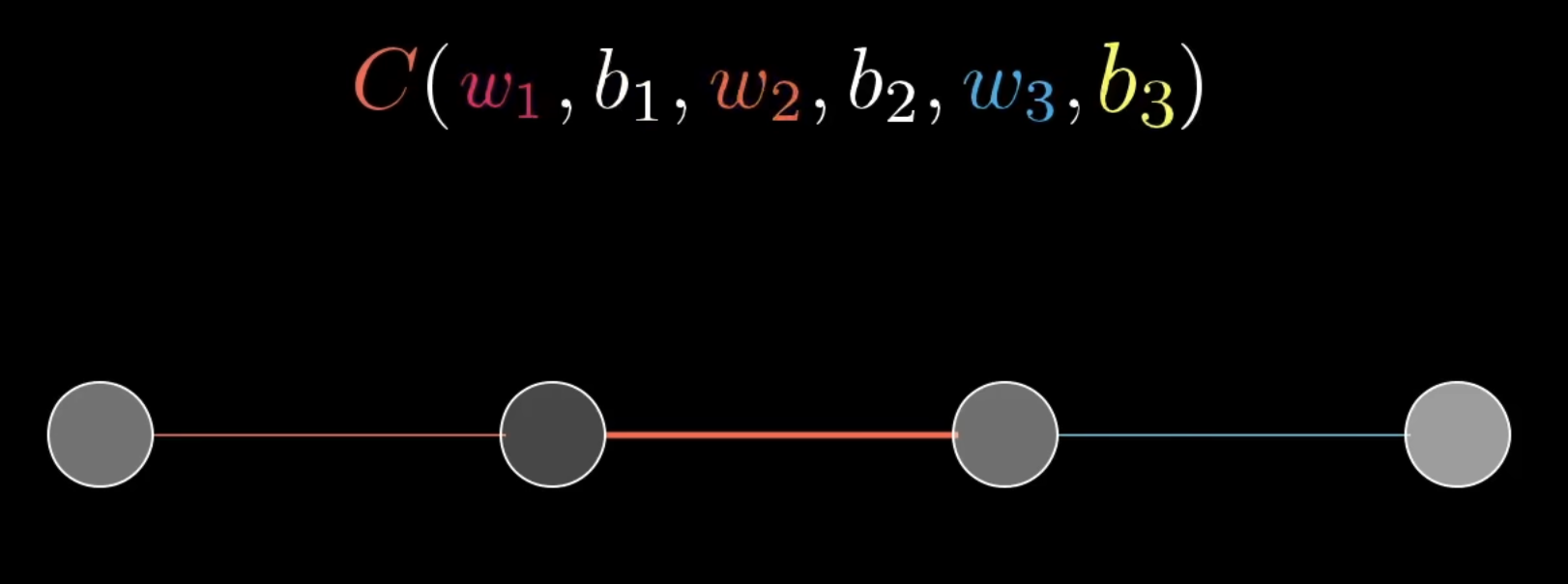
We want to know how sensitive the cost function is to those variables. In other words, we want to know those variables affect the cost function → how model weights and biases affect the loss function. Consider the below:

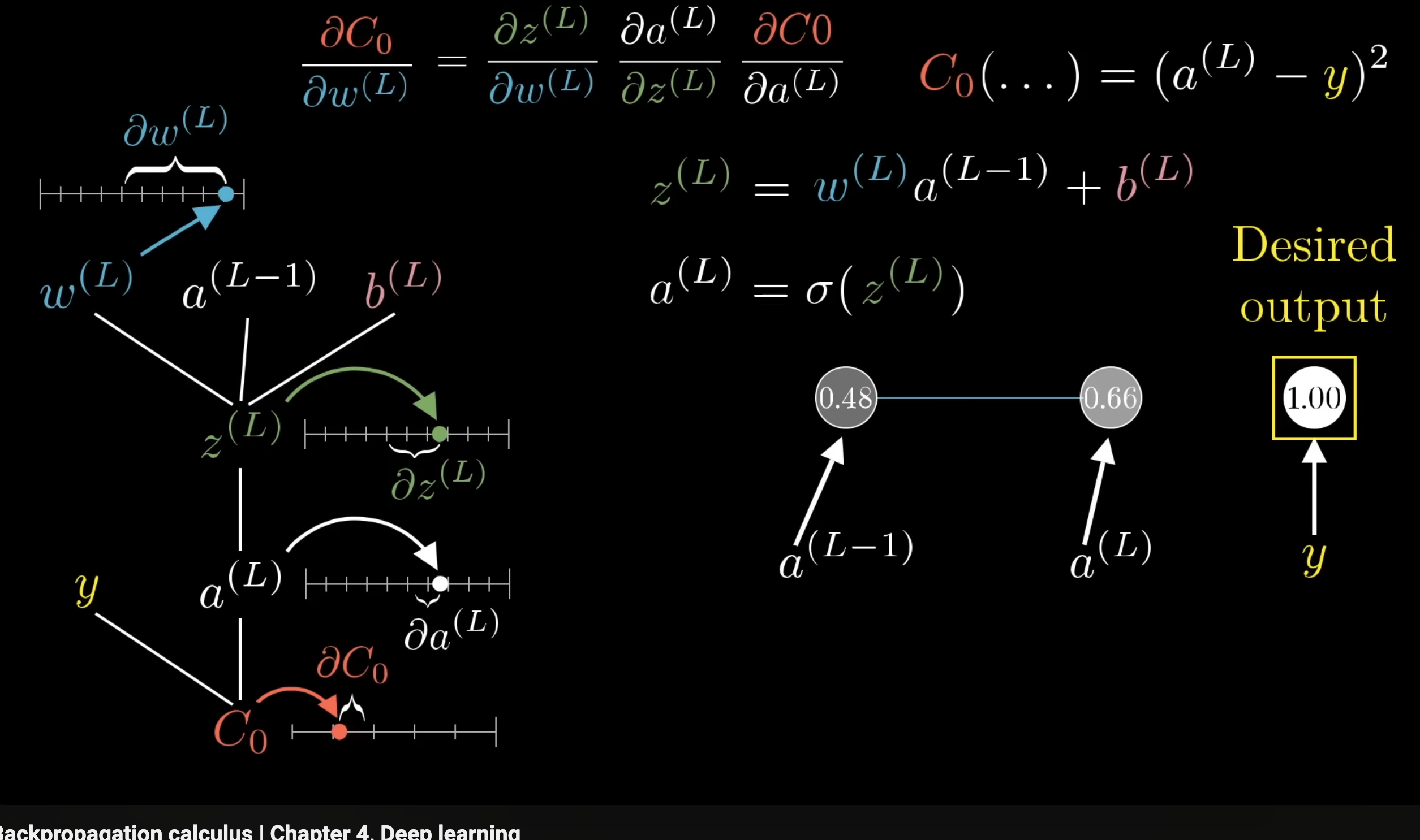
As seen, this is where the chain rule shows itself in backpropagation. Consider:

$$\frac{\partial {\mathcal{C}}_0}{\partial w^{(L)}}=\frac{\partial z^{(L)}}{\partial w^{(L)}}\frac{\partial a^{(L)}}{\partial z^{(L)}}\frac{\partial {\mathcal{C}}_0}{\partial a^{(L)}}=a^{(L-1)}{\sigma }^{\prime }(z^{(L)})2(a^{(L)}-y)$$

This is for the change ins cost with respect to weight in $L$ layer for only one training example. If we wanted to do this over batch, we would so:

$$\underset{\text{Derivative of full cost function}}{\underbrace{\frac{\partial \mathcal{C}}{\partial w^{(L)}}}}=\frac{1}{|B|}\sum _{k=0}^{n-1}\underset{\text{Average of all training examples in the mini-batch}}{\underbrace{\frac{\partial {\mathcal{C}}_k}{\partial w^{(L)}}}}$$

We have $C_i$ as the cost for every layer is different, where $C_0$ is the cost/loss of the last layer, where it is directly compared to the expected labels. This is the only one entry in the gradient vector, which is the objective of backpropagation:

$$\nabla \mathcal{C}=\left[\begin{array}{c}\frac{\partial \mathcal{C}}{\partial w^{(1)}}\\ \frac{\partial \mathcal{C}}{\partial b^{(1)}}\\ ⋮\\ \frac{\partial \mathcal{C}}{\partial w^{(L)}}\\ \frac{\partial \mathcal{C}}{\partial b^{(L)}}\end{array}\right]$$

Right, so this is for a simple simple example, of one neuron per layer. What if we had more neurons? How would you compute $\frac{\partial {\mathcal{C}}_0}{\partial a_k^{(L-1)}}$ , now that there are multiple activations from the previous layer? To do so, we simply sum the derivative over all neurons in the previous layer, so, something like:

$$\frac{\partial {\mathcal{C}}_0}{\partial a_k^{(L-1)}}=\underset{\text{Sum over layer L}}{\underbrace{\sum _{j=0}^{n_L-1}\frac{\partial z_j^{(L)}}{\partial a_k^{(L-1)}}\frac{\partial a_j^{(L)}}{\partial z_j^{(L)}}\frac{\partial {\mathcal{C}}_0}{\partial a_j^{(L)}}}}$$

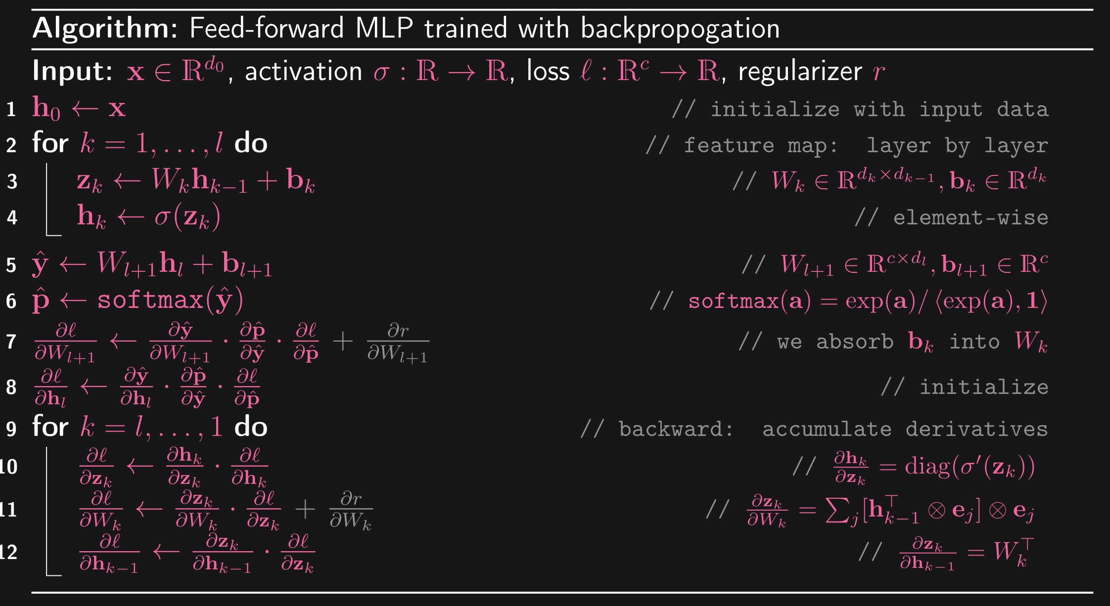
Knowing this, we can now digest the feed-forward MLP trained with backpropagation:

→ Theorem: Universal Approximation NN are often referred to as “Universal Approximation”, since, in theory, they can approximate any function we can imagine, as long as there is some natural world relationship to it. This theorem is effectively stating:

• a feedforward neural network with a single hidden layer containing a finite number of neurons can approximate continuous functions on compact subsets of ${\mathbb{R}}^d$ arbitrarily well, under certain conditions on the activation function.
• Activation: The theorem specifies that the activation function σ\sigmaσ must not be a polynomial (almost everywhere) for the neural network to be able to approximate a wide class of continuous functions densely in the space $C({\mathbb{R}}^d)$ (the space of continuous functions on ${\mathbb{R}}^d$).
  • Hence why common ones like $Relu$ are not polynomial functions
• Dense: This means that for any continuous function $f$ in $C({\mathbb{R}}^d)$, there exists a sequence of neural networks with activation function $\sigma$ that can approximate $f$ arbitrarily closely in the supremum norm over ${\mathbb{R}}^d$.
• Riemann Integrability: The activation function $\sigma$ is assumed to be Riemann integrable on any bounded interval for the theorem’s conditions to hold.

Dropout

This is an interesting technique that we leverage in the face of overfitting. Deep neural networks are capable of incredible learning, but this comes at the risk of overfitting. That is, the model can easily pick up and learn relationships that aren’t of interest, or things that we as humans did not see. In such cases, the model loses the ability to generalize, which is the main purpose of ML models! One technique is dropout. Here are the general details:

• For each training mini-batch, keep each hidden unit with probability $q$, where sometimes we will randomly, at that fixed $q$, make the weight’s entry 0
• Doing so will “lose some of the learned relationships” or weaken them, making it less likely to overfit

Batch Normalization

In deep learning, batch normalization is a technique used to improve the training of artificial neural networks by normalizing the inputs of each layer.

• Batch normalization normalizes the input values of each layer by subtracting the batch mean and dividing by the batch standard deviation. This ensures that the inputs to each layer are roughly in the same range and helps in stabilizing the learning process.
• Refer to the Deep Learning Folder for more in-depth information, I’m too tired : /