Lecture 11- finishing BFS, Starting DFS

BFS Application: Testing Whether a Graph is Bipartite

→ (Undirected) Bipartite Graphs and BFS

Recall that a graph is bipartite if the nodes can be partitioned into sets $R$ and $B$ such that each edge has 1 endpoint in $R$ and the other in $B$
Upon first glance, its not always obvious if a graph is bipartite unless it is structured to show this attribute intentionally

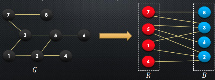
Claim: a graph is bipartite iff it does not contain an odd cycle

How to prove this? We prove this in both directions:

→ odd cycle ⇒ not bipartite
- Suppose for the sake of contradiction, that there $\exists$ an cycle of odd length: $v_{1}, v_{2}, ..., v_{2 k + 1}, v_{1}$
- WLOG, suppose that $v_{1} \in R$ , this then means that $v_{2} \in B$
- If we continue this until $v_{2 k + 1}$ , we will notice that $v_{2 k + 1} \in R$
- But, $v_{2 k + 1}$ is adjacent to $v_{1}$ , and in order to be bipartite, they cannot both be in $R$
- Therefore, arrived at a contradiction → qed
← all cycles have even length ⇒ bipartite
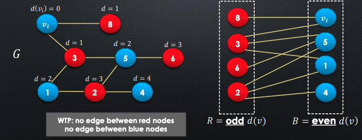
- Let $v_{i}$ be any node, and $d (v)$ to be the distance from $v_{i}$ to $v$
- We partition the rest of the nodes by even vs odd distances to $v_{i}$

Claim: if there were any edges between red or blue nodes, there would be an odd length cycle.

To prove this, we can:

WLOG, suppose for contradiction $(u, v) \in E$ where $u, v \in R$ are red nodes
Since they are red, $d (u)$ and $d (v)$ from $v_{i}$ are both odd
So, what if we did have an edge between the 2 red nodes $u$ and $v$ ? We would then obtain an odd-length cycle.

With the information above, we can contruct an algorithm for testing bipartitness

def Bipartition(adj[1...n]):
	colour[1...n] = [white, white, ..., white]
	dist[1...n] = [infinity, infinity, ..., infinity]
 
	for start in 1...n:
		if colour[start] == white:
			BFS(adj, start, colour, dist)
 
	for edge in adj:
		let u and v be endpoints of edge
		if (dist[u]%2 == dist[v]%2):
			return NotBipartite
	
	B = nodes u with even dist[u]
	R = nodes u with odd dist[u]
	return B, R

In the beginning, we create 2 lists: (1) for the starting colours of all nodes (2) distances from v_i
Then, we iterate over each node, and if white, we will perform a BFS on it. This is in case there are multiple components of the graph
- A bipartite graph can be unconnected
- An unconnected graph is bipartite if its components are bipartite
- Will only be one BFS run if the graph is connected
BFS calculates the distances for each node
This is a modified BFS → it re-uses the same colour array, same distance array
Once the entire graph has been explored, we will go trhough all edges in the graph, and check if the distances to each of the endpoints are both odd or even
- If so, then the graph is not bipartite
At the end, return the 2 partitions of nodes → $R$ and $B$ based on even or odd distance

→ What is the runtime of this algorithm?

Although we have BFS run inside of the for loop, they collectively will visit each node inside of the graph. So, this is just a $O (n + m)$ work. Then, we iterate over all edges comparing the end nodes. We know there are $m$ edges and so, this is a $O (m)$ operation. Lastly, we are constructing $B$ and $R$ which is $O (n)$ . So, overall, the runtime of this algorithm is $O (m + n)$ .

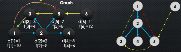
Depth-First Search (DFS)

Like the name suggests, instead of visiting all of the adjacent neighbours, we will visit a neighbour, and keep visiting one neighbour until we can no longer move on
DFS uses a stack (or recursion) instead of a queue
We define predecessors and colour vertices as in BFS
It is also useful to specify a discovery time $d [v]$ and a finishing time $f [v]$ for every vertx $v$
We increment a time counter every time a value $d [v]$ or $f [v]$ is assigned
We eventually visit all the vertices, and the algorithm constructs a DFS forest

Here is the DFS algorithm (should be very familiar for you):

global variables:
	pred[1...n] = [null, null, ..., null]
	colour[1...n] = [white, white, ..., white]
	d[1...n] = [0,0,...,0] # discovery times 
	f[1...n] = [0,0,...,0] # finish times 
	time = 0
 
def DepthFirstSearch(adj[1...n]):
	for v in 1...n:
		if colour[v] == white:
			DFSVisit(v)
 
def DFSVisit(adj[1...n], v):
	colour[v] = gray
	time = time + 1
	d[v] = time
 
	for each w in adj[v]:
		if colour[w] == white:
			pred[w] = v
			DFSVisit(w)
 
	colour[v] = black
	time = time + 1
	f[v] = time

Let’s analyze the DFS algorithm
In DFS, things like pred and colour need to be shared in every DFS call → we could make this pass by reference, but it is easier to make these things global variables
We create d and f as our discover and finish times
We have DepthFirstSearch as the outer function, since this is needed if our graph is directed or has multiple components. If the node is unvisited (white), we will call dfs on it
The actual DFSVisit function is the one performing the depth first search
We mark the current node we are on as gray, increment the time, and assign this as the current node’s discover time
Then, for each unvisited neighbour node, we will assign their pred as the current node, and call DFS on them
After we have finished our DFS on all neighbouring nodes (a.k.a we have visited all reachable nodes from the current node), we mark the current node as black, indicating we are done processing it
We assign the node’s finish time to time

The above sequence of images demonstrates visually how the DFS works. In BFS, we saw that we constructed a BFS tree for connected graph (and BFS Forest for un-connected graphs). The same happens for DFS. In DFS, pred array induces a forest → here is how it is constructed/looks like:

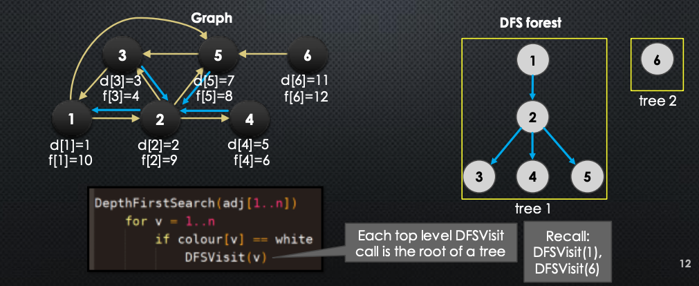
Here are some basic properties to remember:

All nodes start out white
A node $v$ turns gray when it is discovered (also gets a discovery time $d [v]$ ) which is when the first call to DFSVisit(v) happens
After $v$ turns gray, we recurse on its neighbours
After recursing on all neighbours, we turn $v$ black → also gets a finish time $f [v]$
- Recursive calls on neighbours end before DFSVisit(v) does, so the neighbours of $v$ turn black before $v$ turns black

→ So, what is the runtime of the DFS algorithm?

In the beginning, we create the arrays we need to use → $O (n)$
We know that DFSVisit(v) is only called on a node if it is white, so this function is called once per node.
- Each call iterates over all neighbours. Effectively, for each node, for each neighbour, do $O (1)$ work + recurse
Total $O (n + m)$ iterations over all recursive calls → total is $O (n + m)$ runtime

We classify the edges $(u, v)$ in DFS:

If pred[v] = u, then $(u, v)$ is a ==tree edge==: That is u → v is called a tree edge
Otherwise, there are 3 other cases:
- If $v$ is a descendent of $u$ in the DFS forest → ==forward edge==
- If $v$ is an ancestor of $u$ in the DFS forest → ==back edge==
- Else, $(u, v)$ is a ==cross edge==
Note that forward, back, and cross edges are not in the tree. Below is a good diagram of this:

→ Some important definitions:

We use $I_{u}$ to denote $(d [u], f [u])$ , which we will call the interval of $u$
We say “ $v$ is white-reachable from $u$ ”, if there is a path from $u$ to $v$ containing only white nodes (excluding $u$ )
- So, we then say that a DFS call on $u$ will explore all the white-reachable nodes from $u$ . So in the below, nodes 1, 5 and 6 are white-reachable from node $u$ → the nodes that will be discovered from the DFS call on $u$

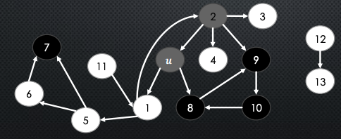
Observe: every node $v$ that is white-reachable from $u$ when we first call DFSVisit(v) becomes gray after $u$ and black before $u$ . This means that $I_{v}$ is nested inside $I_{u}$ . This should be very understandable.

So, as a quick summary, we conclude with the following theorem:

→ Theorem: let $u, v$ be any nodes in the graph. The following statements are all equivalent:

$v$ is white-reachable from $u$ when we call DFSVisit(u)
$v$ turns gray after $u$ and turns black before $u$
discovery/finish time interval $I_{v}$ is nested inside of $I_{u}$
$v$ is discovered during DFSVisit(u)
$v$ is a descendant of $u$ in the DFS Forest

Throughout the DFS algorithm, the DFS inspects every edge in the graph. When DFS inspects every edge ${u, v}$ , the colour of $v$ and relationship between the intervals of $u$ and $v$ determine the edge type. The following table summarizes this nicely:

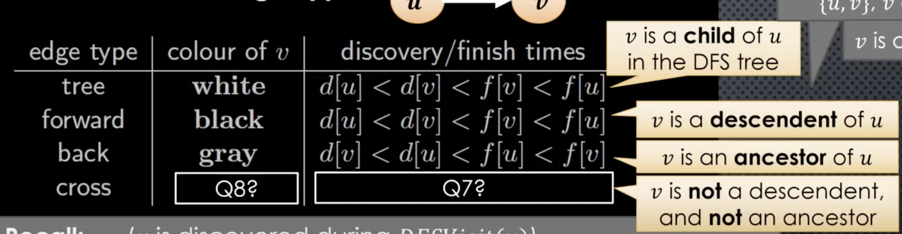
So, what is this saying? Based on the theorem above, consider the edge between $u$ and $v$ . If it is a:

tree edge u→v: then, we know that $v$ is a child of $u$ in the DFS tree, and so, we know that $v$ is white
forward edge: then, we know that $v$ is a descendent of $u$ in the DFS forest. This means that we full process $v$ before returning to $u$ . Hence, it is black
back edge: then, we know that $v$ is an ancestor of $u$ . So, this means that when calling dfs on $u$ , we eventually reached $v$ and it points back to $u$ . This means that $u$ is gray, as it has no completed yet. We’ve discovered $v$ but we have not finished it → so gray
What about cross edge? We do not know, the above theorem is not capable of handling this case. This is because for this, $v$ is neither a descendent or ancestor of $v$ . We need additional information

Useful Fact: Parenthesis Theorem → For each pair of nodes $u, v$ the intervals of $u$ and $v$ are either disjoint or nested. So, there are no intervals with overlaps.

→ Proof:

Suppose the intervals are not disjoint → there is some overlap
Then either $d [v] \in I_{u}$ or $d [u] \in I_{v}$
WLOG, suppose that $d [v] \in I_{u}$
This then means that $v$ is discovered during DFSVisit(u), so, $v$ must turn gray after $u$ and black before $u$ .
So, this means that $f [v] < f [u]$
This means that the intervals are nested

With this theorem, we revisit the image above. We can quikcly come to the conclusion that it is not nested → as this would imply that either $u$ is a descendent of $v$ or vic versa. So, they have to be disjoint. The question is, which one is earlier? As there is an edge from $u$ → $v$ , we cannot let the start time of $u$ occur before $v$ , as it would then visit $v$ , making these intervals not disjoint. We revisit the above diagram to better visualize this:

Application of DFS (or BFS)

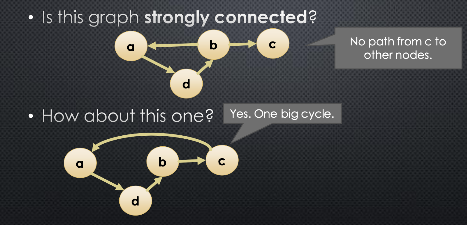
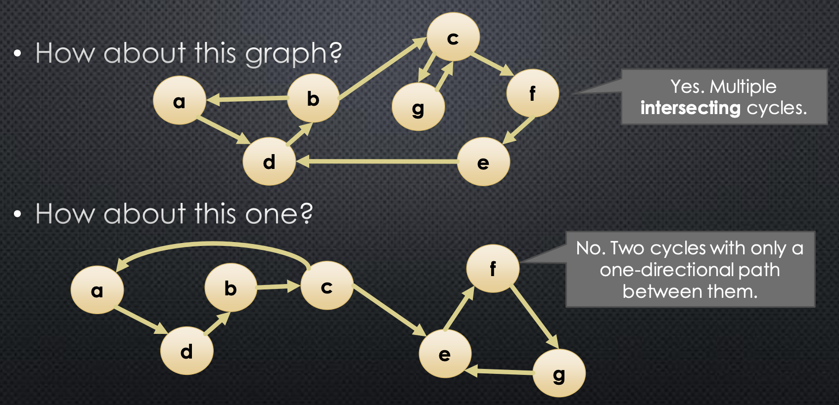
→ Strong Connectedness

In a directed graph:
- $v$ is reachable from $w$ if there is a path from $w$ to $v$
- We denote this path with $w ⇝ v$ whereas an edge would be denoted $u \to v$
A graph $G$ is strongly connected iff every node is reachable from every other node. More fomally → $\forall_{w, v} \exists w ⇝ v$

Below we give an example:

So, what do we gain from knowing that a graph is strongly connected? For example, we can start a graph traversal at any node, and know the node will reach every other node. Without strong connectedness, if we want to run a graph traversal that reaches every node in a single pass, we would need to do additional processing to determine an appropriate starting node.

Another instance of this being useful is as a sanity check. Suppose we want to run an algorithm that requires strong connectedness and we believe out input is strongly connected. It may be advised to verify that our input is indeed strongly connected. So, perhaps we can use DFS to accomplish this? We ask ourselves:

How to use DFS to determine whether every node is reachable from a given node $s$
- Perform a DFS from node $s$ and see if every other node turns black
How to use DFS to determine whether $s$ is reachable from every node
- This is interesting. The naive approach would be to perform a DFS on every other node, and see if all of them are able to reach $s$ . This is far from ideal, as it results in a $n \times O (n + m)$ run time.
- A clever, and $O (n + m)$ way of doing this is to reverse the direction of all edges. Why would this work? If there was a path from arbitrary node $v$ to $s$ , then reversing the edges in this path essentially inverts the direction of the path. So now, we need to see if there is a path from $s$ to $v$ in graph, say $G_{R}$ — graph reversed, which becomes the first bullet-point.

Here is what the algorithm will look like:

def isConnected(G):
    V, E = G
    (color, d, f) = DFSVisit(V[0], G)
    
    for i in 1...n:  
        if color[V[i]] != black:
            return False
    
    H = reverseGraph(G)
    (color, d, f) = DFSVisit(V[0], H)
    
    for i in range(1, len(V) + 1):
        if color[V[i]] != black:
            return False
    
    return True

How would we go about reversing the adjacency array? We will show this for the adjacency matrix. Turn out, its just computing the transpose of the adjacency matrix.

This is actually slightly expensive. We will need to look into each cell to know how to flip → this is $O (n^{2})$ complexity. What about reversing adjacency lists? Very straightforward. We construct a new adjacney list, and iterate through every list in the original one. Something like:

def TransposeLists(adj[1...n]):
	newAdj = new array of n lists
	for u = 1 ... n:
		for v in adj[u]:
			newAdj[v].insert(u)
	return newAdj

The runtime of this is $O (n + m)$ . So, this is prefered as using this will not affect the total runtime of checking if a graph is strongly connected. Therefore, the above algorithm, using a adjacency list, as run-time $O (n + m)$ .

💻 Allan Yin's Blog

Explorer

Lecture 11- finishing BFS, Starting DFS

BFS Application: Testing Whether a Graph is Bipartite

Depth-First Search (DFS)

Application of DFS (or BFS)

Graph View

Table of Contents

Backlinks