Chapter 7 - Transformer Architecture Part 2

edit: This note was made before the other transformer one. This is more visual explanation. It’s important to first read that one before this, as RNN’s are important

This chapter goes over the transformer architecture, and in particular, how it addresses the downfalls of residual networks and how transformers work. A Transformer is a special kind of neural network and it is the core invention underlying the current boom in AI.

Word Embeddings

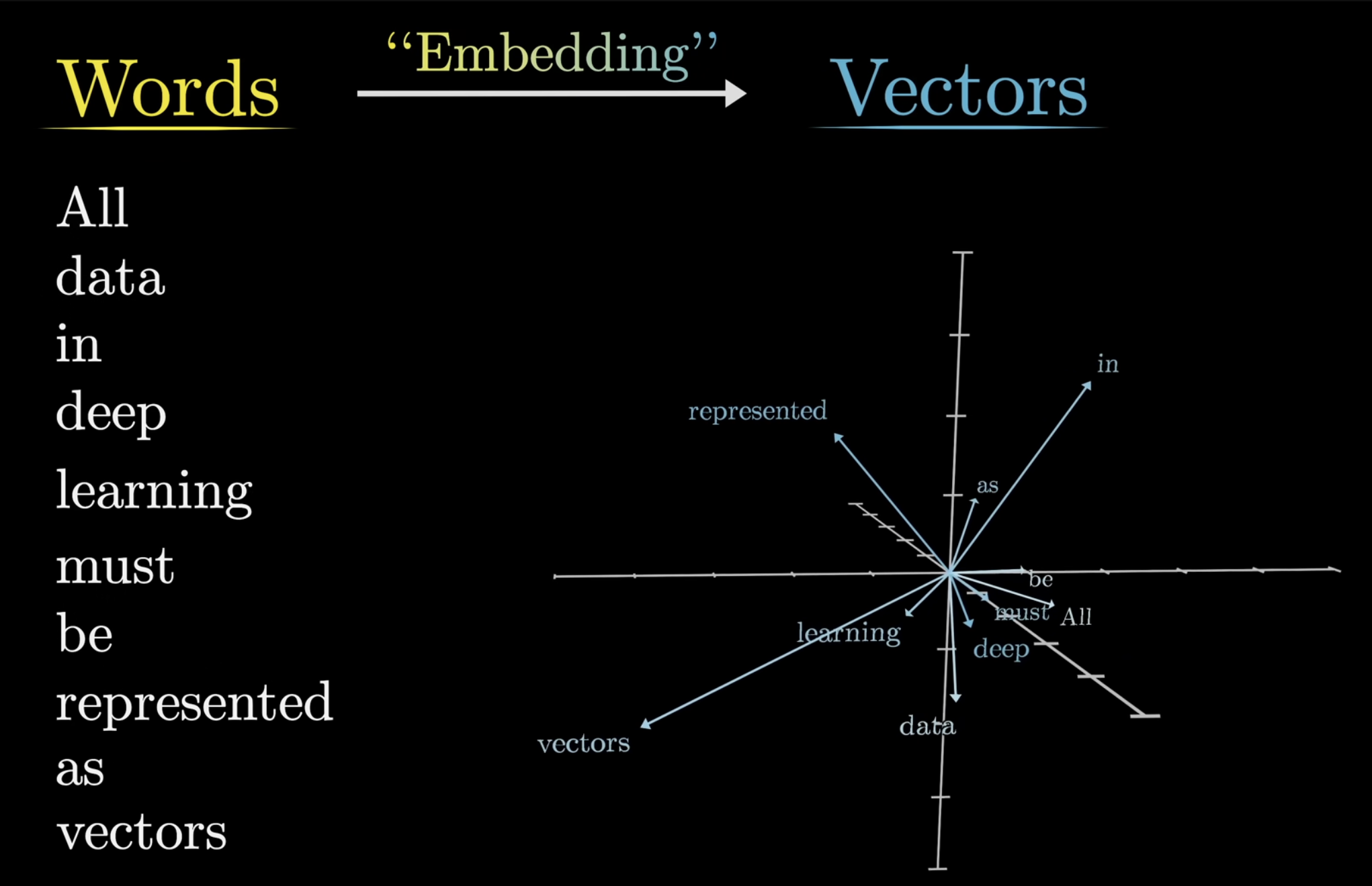
For now, let’s try and understand transformer models through the lens of LLM’s, such as GPT3. Let’s consider a text processing example, where the inputs to the model are text snippets. The first step in these models is to break up the input into little chunks, and then make those chunks into little vectors. Each of these chunks is called a token, which you may recall when you are charged per token when using OpenAI API calls.

For simplicity, we’ll largely assume each word is its own token, which is not always the case, but its easier to think about the embeddings this way. To start, our model has a pre-defined vocabulary, some list of all possible words ~ 50k. The first matrix we will encounter, known as the embedding matrix, has a column for each of these words. Let’s denote this matrix $W_E$ where the values begin random, but are learned over time. This process of vectorizing a word has been very common in machine learning, and we often refer to this as embedding a word. Once words have been vectorized, we can represent them in some higher dimension, as so:

For example, a word embedding in GPT3 has 12,288 coordinates (honestly mind blowing) which is beyond any human capacity to imagine. Now, while in concept this is failrly understandable, it is actually quite amazing.

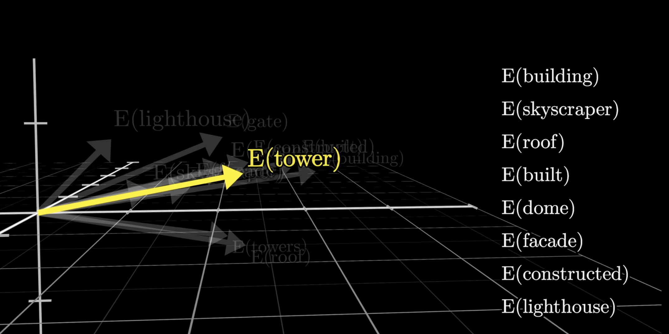
Take this for example, via the embedding, the corresponding vectors for these words happen (not through coincidence) to be grouped in a similar area. The general trend is that words.

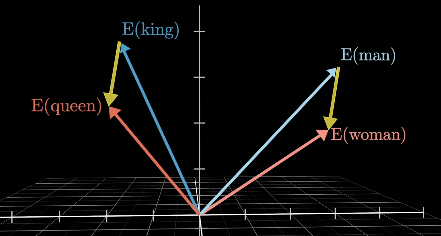
This is truly astounding. While the vector difference is not exact, its roughly similar. The vector queen is actually a bit farther, but that is because in data, the word “Queen” is often used for different semantic reasons than “King”.

Context

Here is a general view of what a transformer looks like:

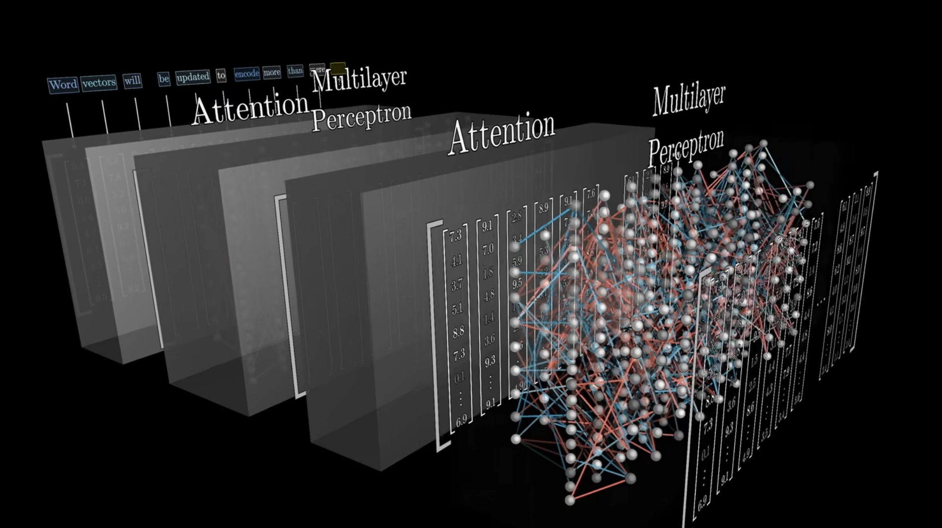
The magic of Transforms come from the attention mechanism. In neural networks, there is the issue of certain information being lost. We first saw recurrent neural networks. Transformers aim to solve these even better. In the above image, we have attention layers. But, what is attention? We’ll dive deeper into this later, but it solves a fundamental problem that we encounter in NLP. Namely, how can we process english language? In an input sentence, the semantics of a word are highly dependent on the surrounding words in the sentence. So, when we are updating weights that correspond to that word in the vector embedding, how can we make it so, the “learning” of weights is in relation to the other words? This is the purpose of attention. Things like the position of the word in the sentence, the presence of other words, etc.

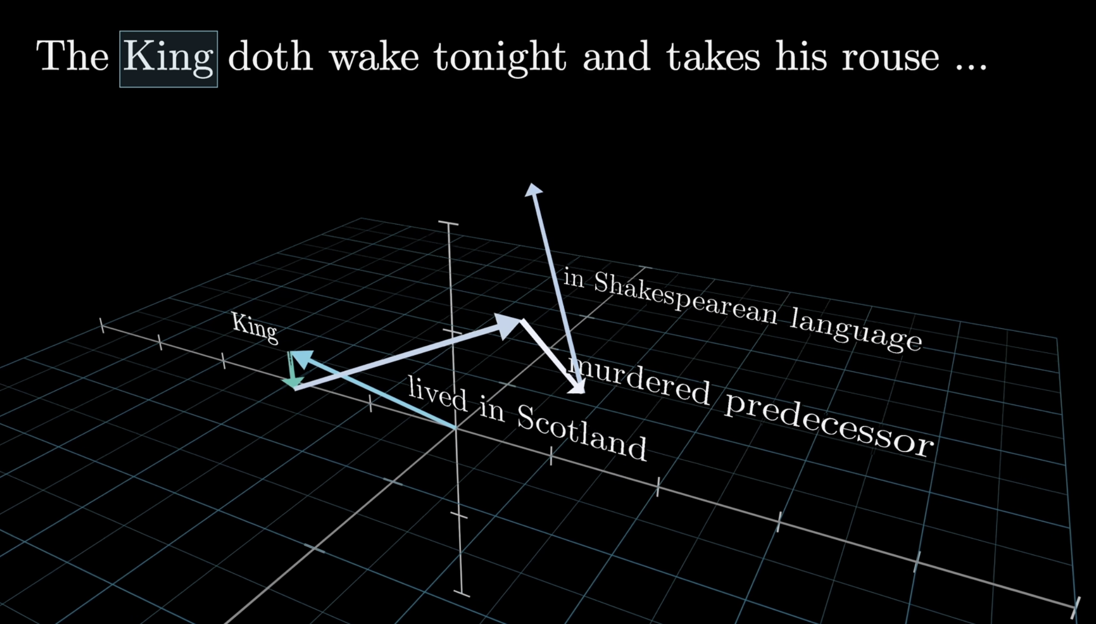Much like the vector difference between words above, we can add these “semantic differences”, which in each direction the vector is pulled (and hence the semantic meaning is modified), the words “definition” is changed. In short, when building models that are supposed to somehow predict what word comes next, the goal is to somehow empower the model to incorporate context efficiently.

The primary goal of this attention block is to enable each one those word/token vectors in the input, to soak up a meaning that is much more rich and specific that mere individual words could represent. The network can only process a fixed number of vectors at a time, this is known as the context size, which for GPT3, was 2,048. This context size effectively limits how much text the transformer can incorporate when its making a prediction of the next word → fun fact: this is why long conversations with early versions of ChatGPT often gave the feeling that the chatbot was losing the thread of the conversation as it became lengthy

We’ll come back to really focus on attention, but before then, let’s quickly examine what happens at the end of the network. Recall that the output is a probability distribution over all tokens that might come next. For example:

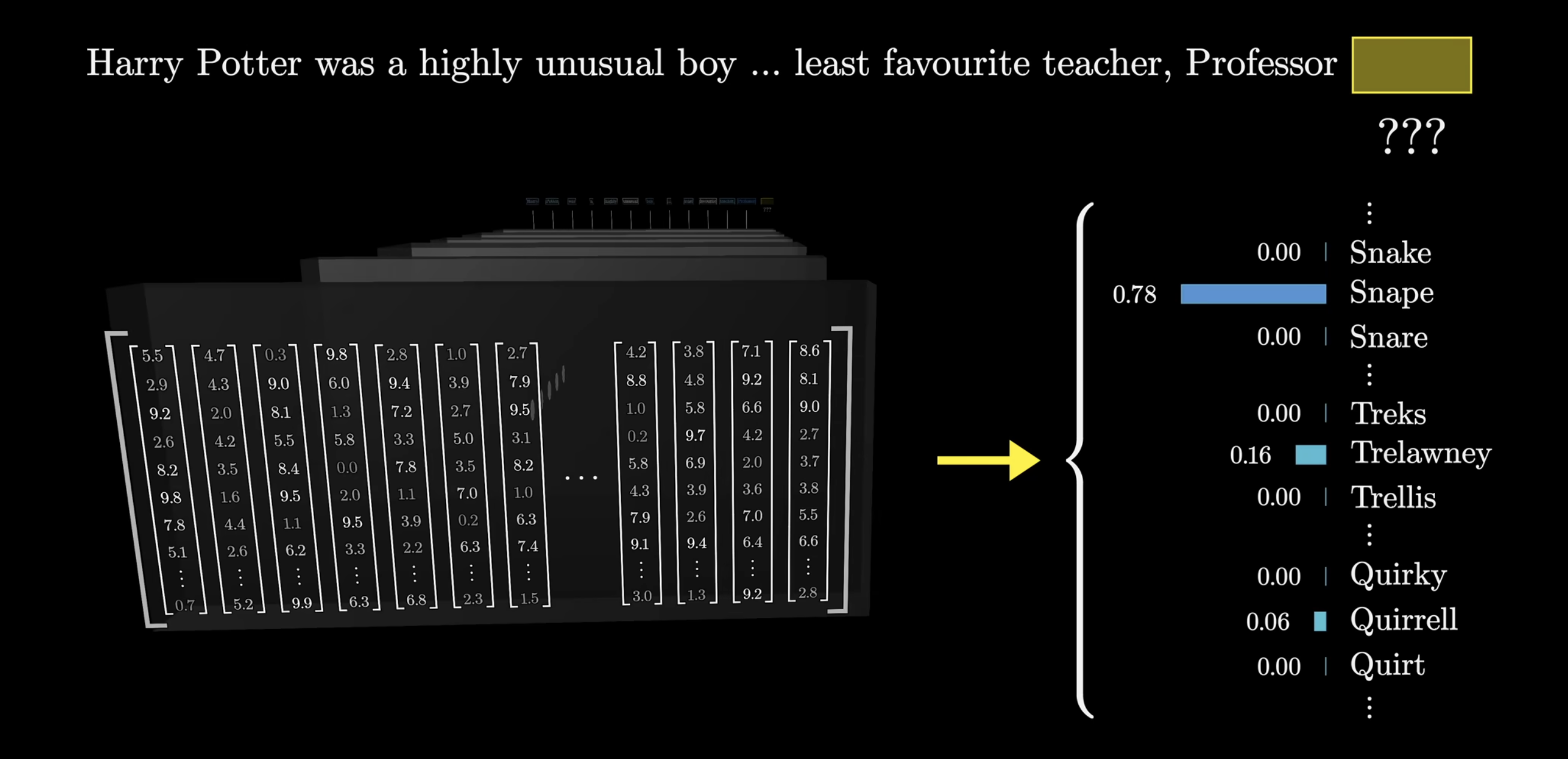
So, given the above, the model would presumably assign a high probability to the word Snape. This itself involves a couple of steps:

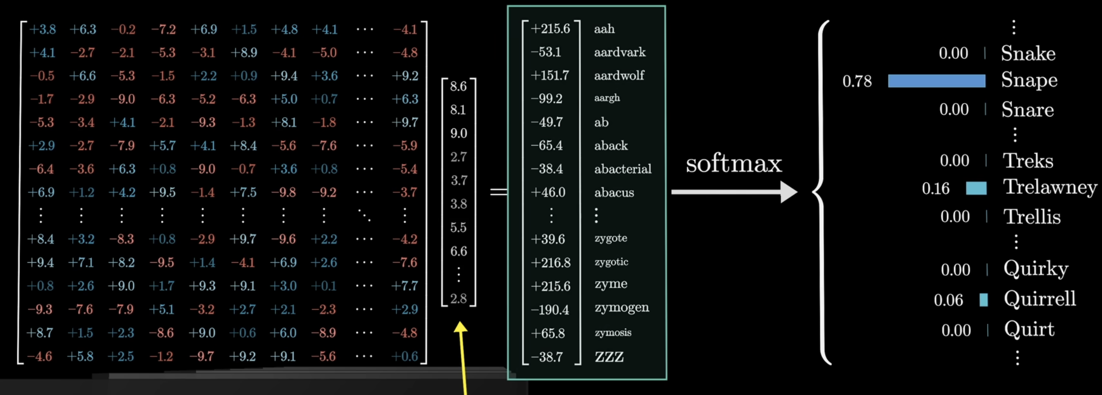
First, we have another matrix that matches the very last vector in the context, to a list of 50k values, one for each token in the vocabulary. We then normalize this into a probability distribution, softmax above. But, isn’t kind of weird to only use the last embedding in the above? In the last layer of the network, we have thousands of other context vectors, that … just sort of sit there. We’ll see this later as well. We call the matrix above the Unembedding matrix: $W_U$, which, like the embedding matrix, is randomized in the beginning, but later parameters are learned. In order to multiply the context vector, which is just a column of the embedding matrix, the unembedding matrix has dimensions that of the transpose of the embedding matrix.

→ Softmax Quick The idea is, if you want a sequence of numbers to act as a probability distribution, then each value needs to be between 0 and 1, and we need all of them to add up to 1. But, as we know in Deep Learning, the output of these layers is unpredictable: we can get negatives, and definitely won’t sum to 1 → not a probability distribution at all!

• Softmax is a standard method of turning an arbitrary list of numbers into a valid distribution, in such a way that the largest values end up closest to 1 and the smallest, close to 0.

Now, let’s really examine these attention blocks.

Attention in Transformers

Remember, the core function of the model we are studying, is to, given a snippet of input text, predict the next word in this sequence. Attention mechanisms can be hard to understand, so take your time. Let’s first ask ourselves, what is attention supposed to do? Consider the following sentences:

$$\text{American shrew mole}$$ $$\text{One mole of carbon dioxide}$$ $$\text{Take a biopsy of the mole}$$

In each of these sentences, the word “mole” is referring to something different (animal in the first one, quantity in the second, and the skin condition in the third), that can only be understood via the context around the word. But, in the first step of word embeddings, each token is associated with its own initial vector, the vectors for “mole” in all 3 cases, is the same. In the above, we mentioned that the attention blocks to move information encoded in one embedding to that of another, potentially ones that are quite far away (perhaps the input is a chapter of a book, and the the next word depends on everything in the chapter). After the entire network, the computation performed to produce a prediction for the next word, is entirely a function of the last vector in the sequence.

Imagine the input is most of a mystery novel, all the way until the last sentence: “The murderer was …“. To accurately predict the next word, the final vector in the sequence will have to have been updated by all the attention blocks, to represent much more than any individual word, somehow encoding all of the information in the relevant context window needed to predict the next word. Let’s take a look at the computations computed in an attention block

→ Attention Example The book example is too large for us to examine, so instead, consider the input phrase: “a fluffy blue creature roamed the verdant forest”, and suppose for the moment, the only updates we care about is having the adjectives adjust the meanings of the corresponding nouns. This is the beginning of the concept head of attention.

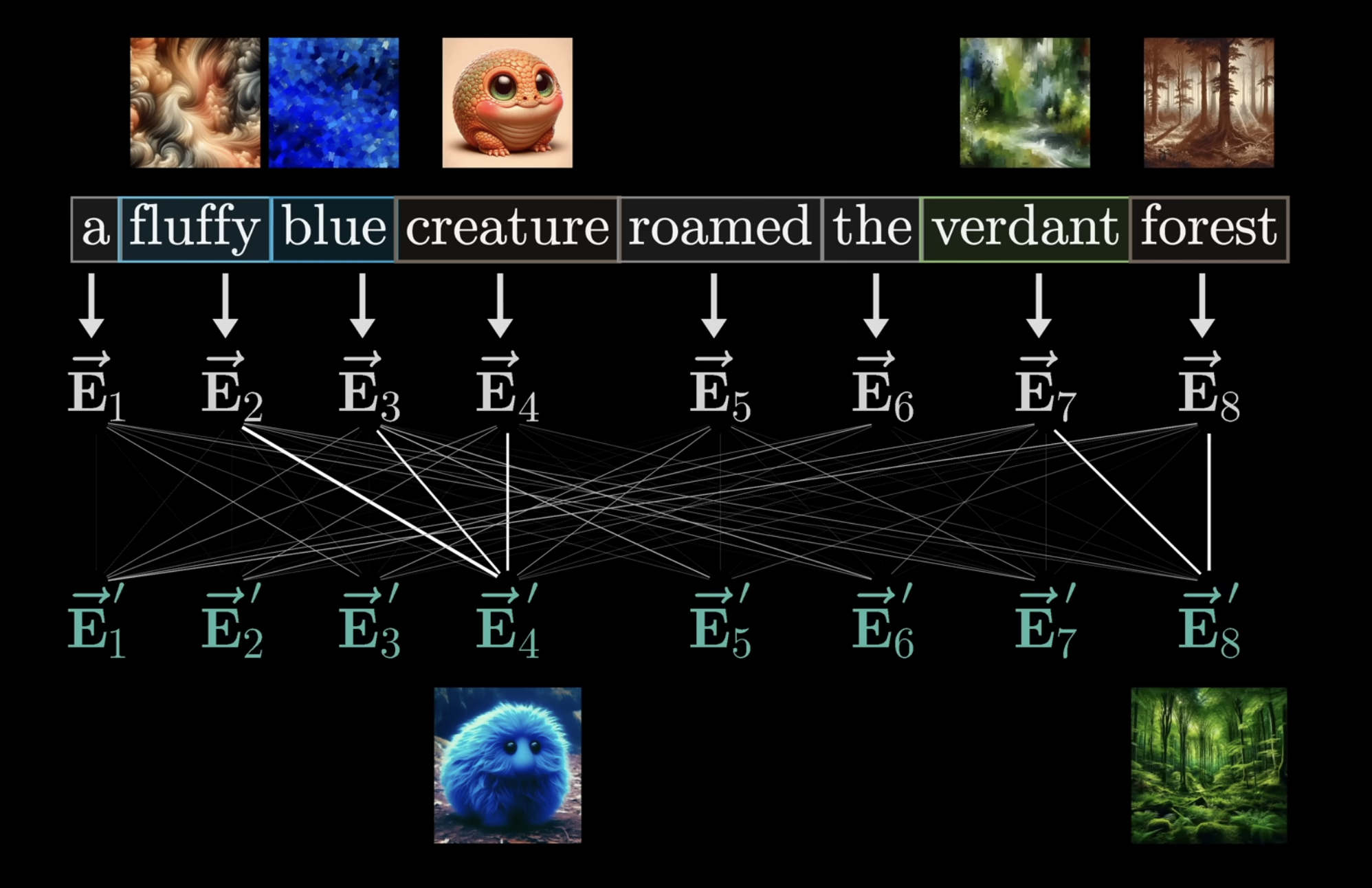
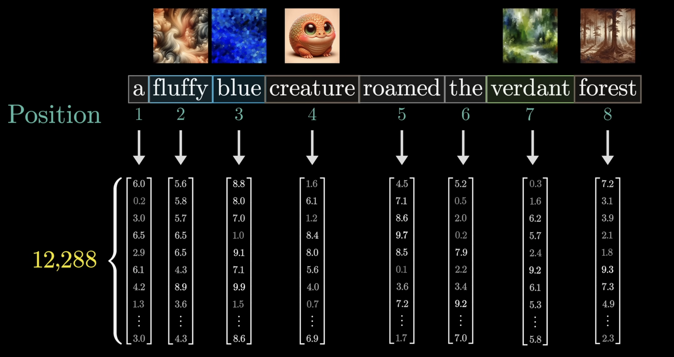In the beginning, each vector embeds the word as well as the position of the word in the context. We denote each of these vector embeddings $E_i$ for each column vector $i$. To goal is have a series of computations to produce a new set of refined embeddings, where for example, the vectors corresponding to the nouns, have ingested the meaning from their corresponding adjectives. These processes will look like many matrix vector products of weights and data. Again, remember this “adjective noun” is purely an example, where in reality, the true behaviour is much harder to parse (true for all of deep learning) since its black box parameter tweaking.

An important concept to know is the idea of a query vector. Imagine if each noun were to ask “what adjectives are there in front of me”, we would want “fluffy” and “blue” to respond with a yes. This question is encoded into a vector, called the query vector. This query vector is obtained by multiplying the embedding vector $E_i$ with some matrix $W_Q$. We’ll do this for all embedding vectors. The weights in $W_Q$. We know that multiplying a matrix is like performing some linear transformation. In particular, imagine this actions as:

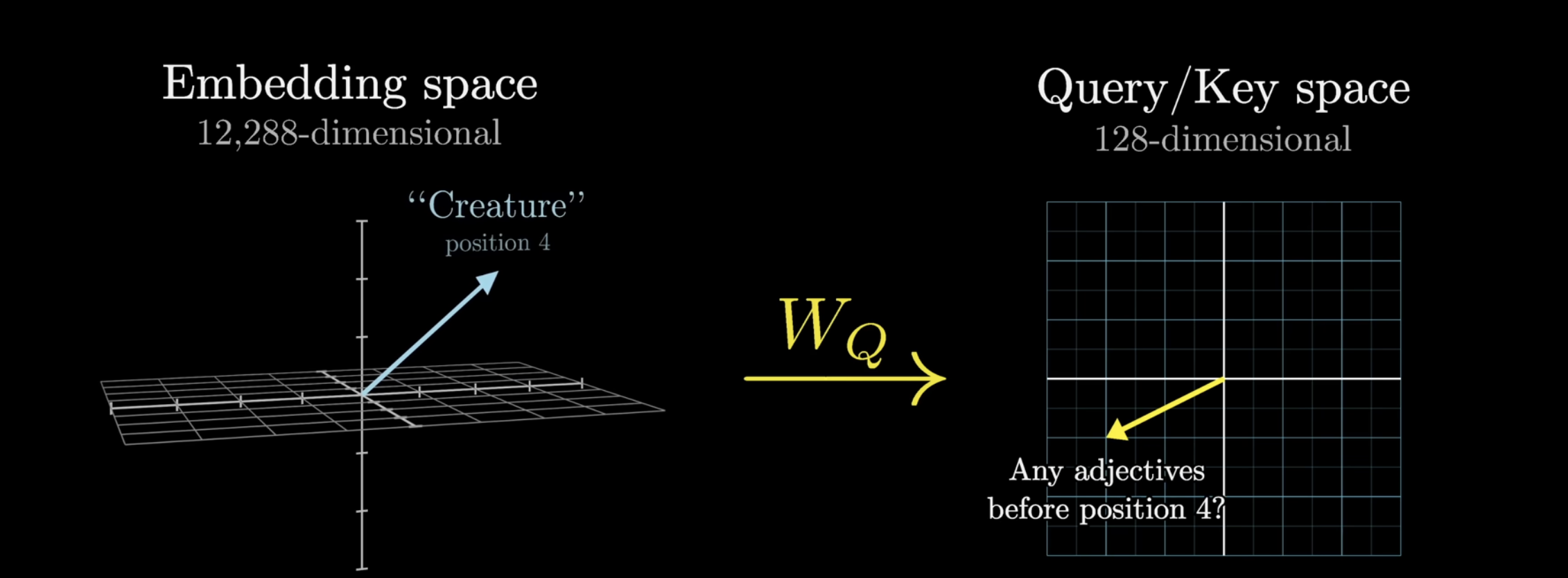
That is, the output query vector is also in its own 128-dimensional space. What will this do for non-nouns? Who knows, we’re only focused on this example scenario for nouns. At the same time, there is another matrix $W_K$ that is called the key matrix, which we also multiply by every embedding vector, to create a sequence of vectors $K_i$ that we call the keys. Conceptually, think of the keys as the answers to the query vectors: “Any adjectives in front of me” → “I’m an adjective in front of you!”, etc. We think of the keys matching the queries when they closely align with each other, in other words, when we map the key and query to their vector space, they generally align. We know that the dot product of 2 vectors are oriented in the same general direction if the 2 vectors are so as well.

• So, we take the dot product of every key with every query, resulting in a table (larger circles represent larger dot product):
• 

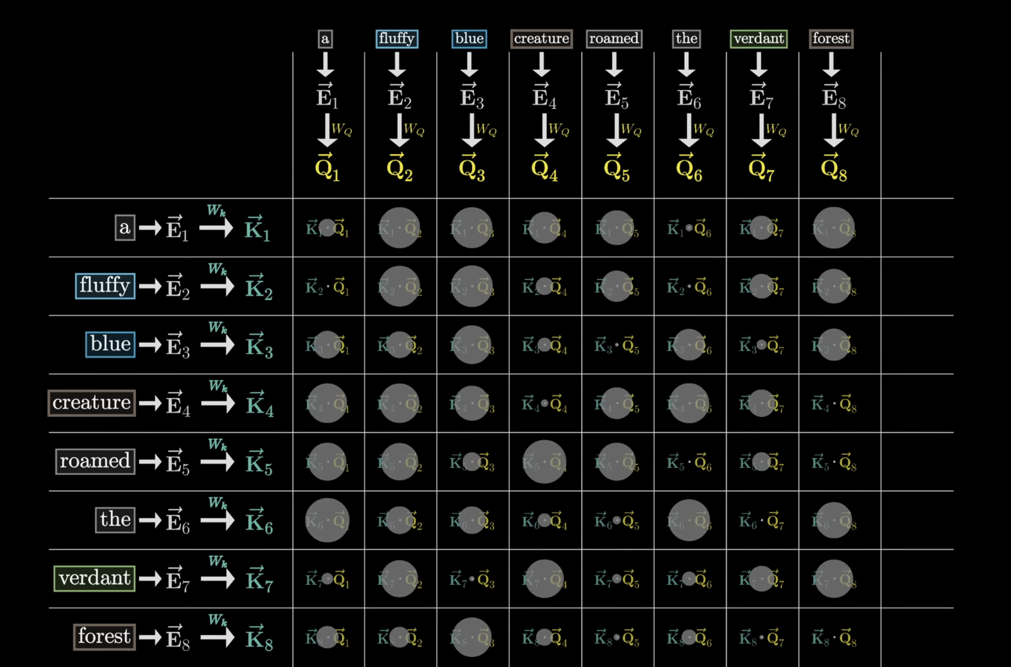
The larger dot product, the more closely the keys align with the query → some large positive number. In machine learning lingo, we would say the embeddings of fluffy and blue attend to the embedding of creature. If the dot product is some small negative value, hence no relation. Now, in each of these columns, the values can range from negative infinity to positive infinity, we want them to be between 0 and 1 → softmax is applied to achieve this. Now, each number in the above grid is between 0 and 1, and we can think of this as “how important is the word on the left to the word on top?” This grid is called an attention pattern. We can express this entire concept very succinctly:

$$\text{Attention}(Q,K,V)=\text{softmax}(\frac{Q{K}^T}{\sqrt{d_k}})V$$

Here:

• $Q$ and $K$ represent arrays of the query and key vectors respectively
• Inside the softmax, the numerator is a very compact way to express the grid
• We divide by root of $d_k$ which is the dimension in the key query space, for stability purposes
• The softmax is understood to be applied column by column
• We’ll see the $V$ term later

So, we know the purpose of the model is to predict the next word/token that is to come in the input. During training, it is actually helpful to do this for every subsequence of the input:

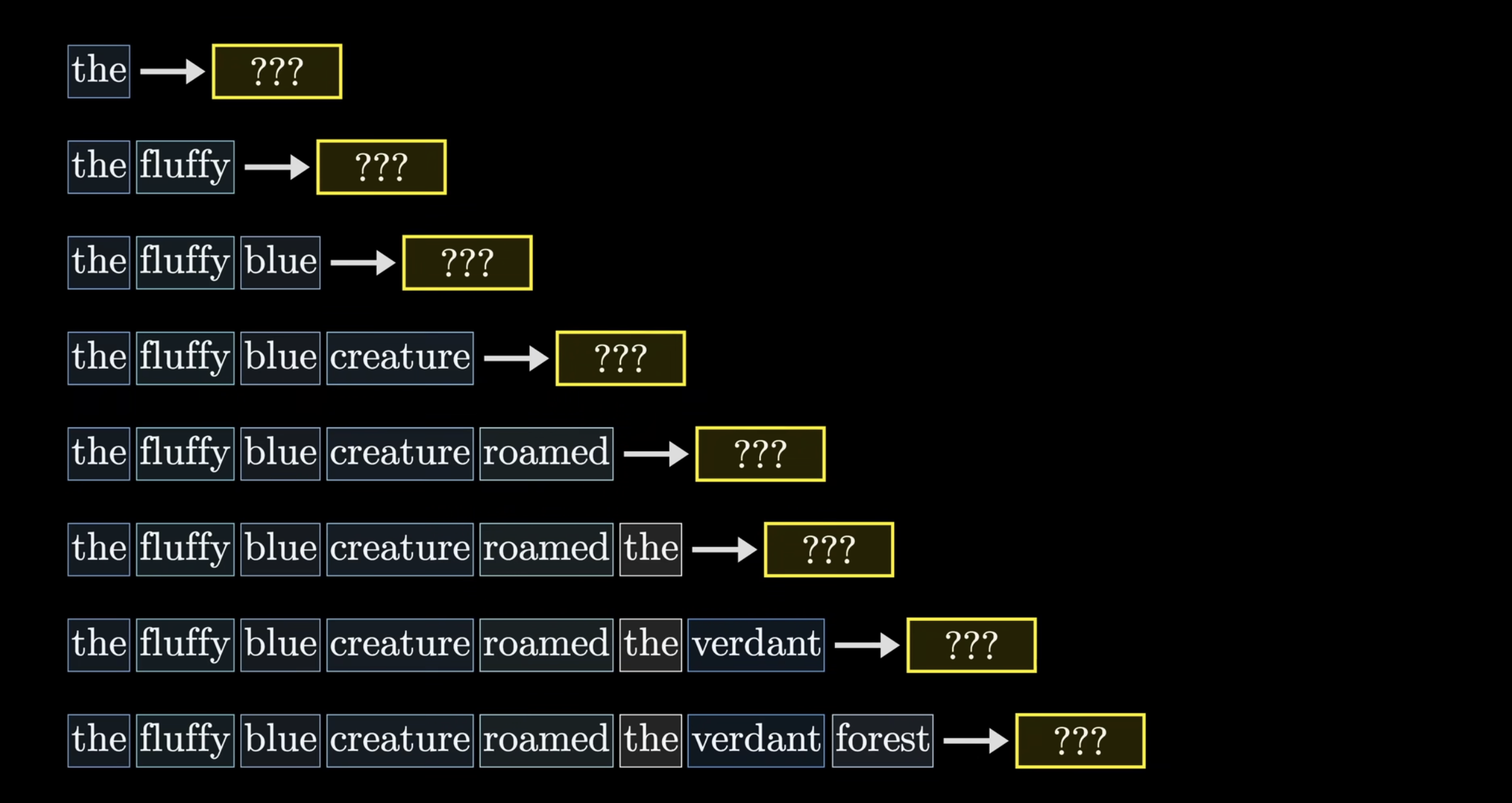
This is nice in that, what would have been one example, can serve as multiple. Since we’re doing this, we need to adjust the attention pattern. What this means is that, given each subsequence trains the model, we never want to allow later words to influence earlier words, since they could “give away” the answer. So in the attention pattern grid, the bottom left half of the grid should be 0. We achieve this by setting those values to negative infinity before performing the softmax → this is called masking. Something important to reflect on is the size of the attention pattern, which has size equal to the square of the context size. This is why context size can be such a bottle neck for LLM’s, and scaling is difficult.

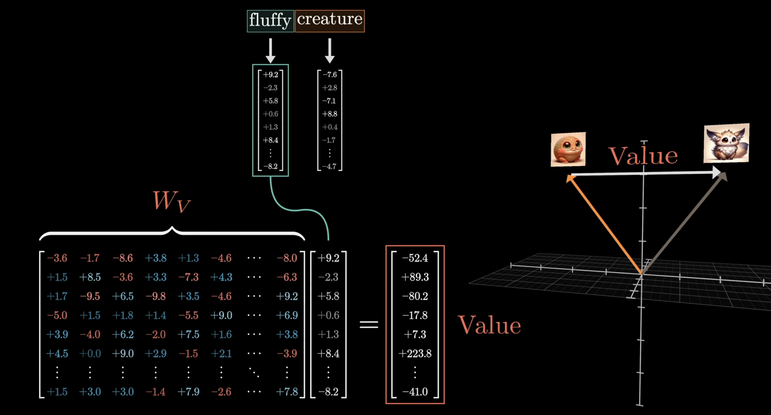
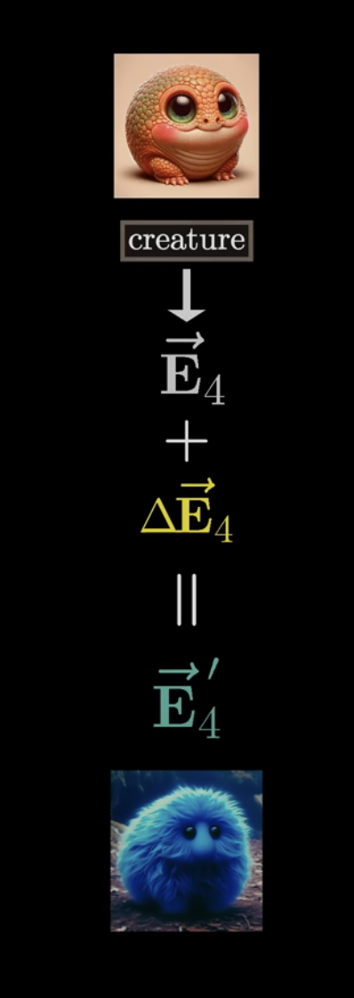
Ok, great, so now we have computed this attention pattern. Now, we actually need to update the embeddings, allowing words to pass information to other words they are relevant to. For example, we somehow want the embedding “fluffy” to cause a change to “creature”, that moves it to a different part of the vector embedding space, that encodes “fluffy creature”. The simple way would be to introduce yet another matrix, called the value matrix:

We can repeat this in our attention grid:

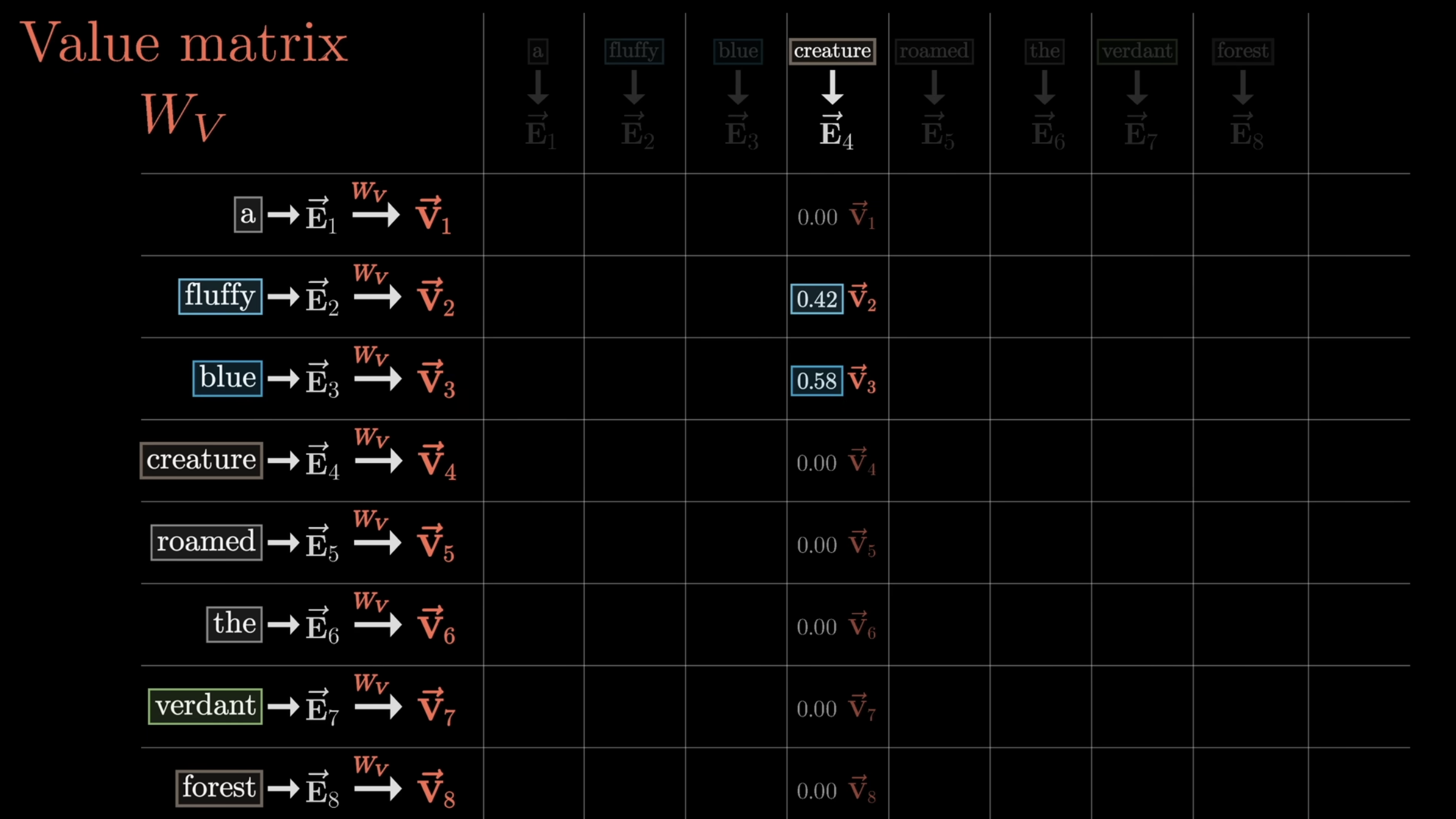
So, we multiply each embedding by value matrix to obtain value vectors. Then, we sum the product of each value vector with the corresponding weight in the column, to obtain $\Delta E_i$ which we add back to the original embedding.

Zooming out, this entire process is whats known as head of attention. This process is parametrized by 3 distinct matrices: Query, Key, and Value. Now, consider the diagram:

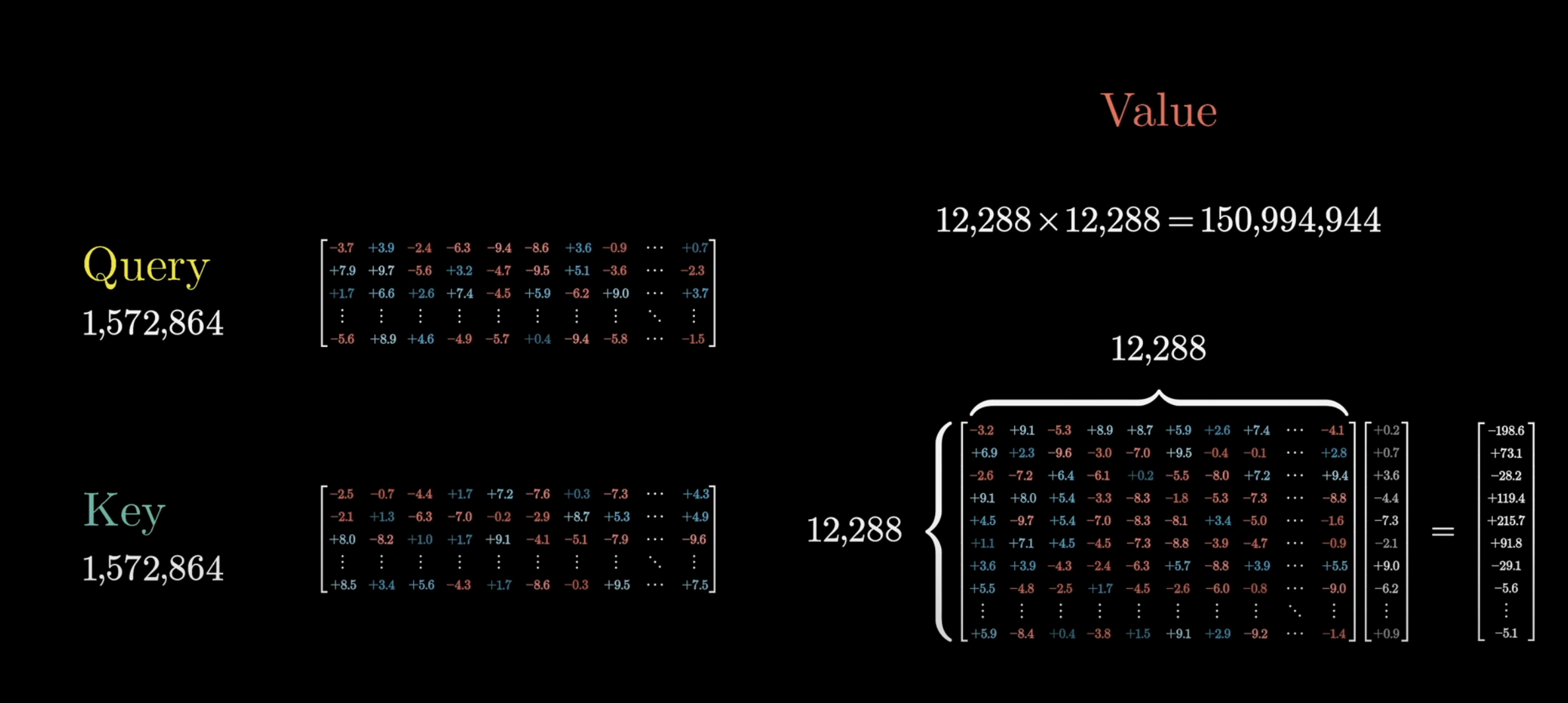Now, the value map is much larger than the query and key ones, and we have devoted orders of magnitude more. This is fine, but in practice, inefficient. Instead, we want # of Value params = # Query params + # Key params. To do this, we split the value map into the product of 2 smaller matrices. So, the 12,288 x 12,288 matrix now becomes the product of 12,288 x 128 and 128 x 12,288.

To be clear, every thing so far is called self-attention, which we need to distinguish from something called cross-attention. Cross-attention involved models that process 2 distinct types of data, like text and images (vision transformers → for final project). A cross-attention head looks almost identical, where the main difference is the key and query maps act on different data sets.

So, thats attention! In a transformer model, we would do this attention mechanism many many (~10,000) times. We focused on the super simple example, of adjectives influencing nouns, but of course, there are other of other ways in which meaning can be influenced from context → “they crashed the car”, lots of contex influecing what the car looks like “beat up, broken, etc.”.

So, this has been single head of attention, there is also multi-head attention. The full attention block inside a transformer consists of multi-headed attention, where we run a lot of these operations in parallel, each with its own key, query, and value maps → GPT3 uses 96 attention heads in each block, which is amazing. One attention block is already a lot to keep track of, so 96 concurrent ones is honestly crazy. So each one of these 96 heads produces a $\Delta E_i$, which are then all summed up and added to the original embedding. This modified embedding vector would merely be a single slice of the output of the attention block.

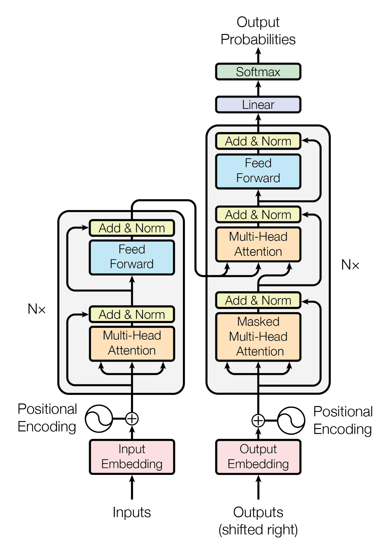
This is then passed through a dense layer of neurons that we’ve seen in dense neural networks. I’ll make some extra notes for this later on. The full transformer architecture is as follows:

Let’s make notes on this:

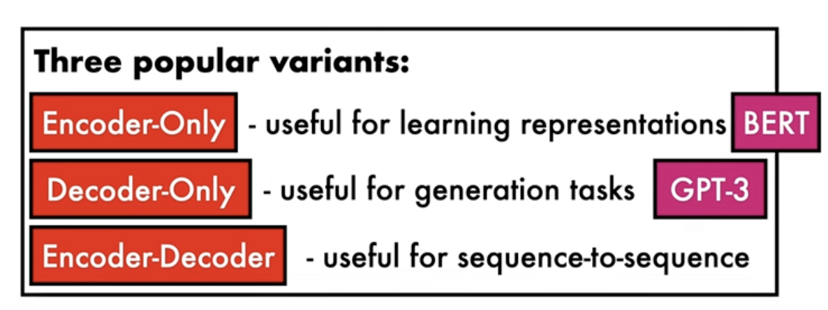
• Left side is encoder → observe that we use residual connections before the dense layer and before the attention block → the encoder is not predicting the next word, rather, the encoder is primarily used to generate the new token embeddings that now contain “context”
• Right side is decoder → the part where we shift right, is the above image of the each subsequence of the input (the embedding vectors anyways). The decoder is used to predict the next word in the sequence, after the encoder has finished:
  • The decoder in a Transformer model requires two types of inputs to generate the output sequence:
    • Encoded Output: The context-aware embeddings produced by the encoder.
    • Output Embeddings: The embeddings of the tokens generated so far in the target sequence (shifted right).
      • Generation Context: The output embeddings represent the previously generated tokens in the target sequence. During training, these are the correct tokens shifted right. During inference, these are the tokens generated so far.
      • Autoregressive Prediction: This enables the decoder to generate the next token based on the tokens it has already produced, maintaining the autoregressive nature of the sequence generation.

Vision Transformers

Briefly mentioned in class. This link is useful: https://www.youtube.com/watch?v=j3VNqtJUoz0&ab_channel=DeepFindr

• Will likely want to use this when building model for final project
• This is an example of an encoder-only

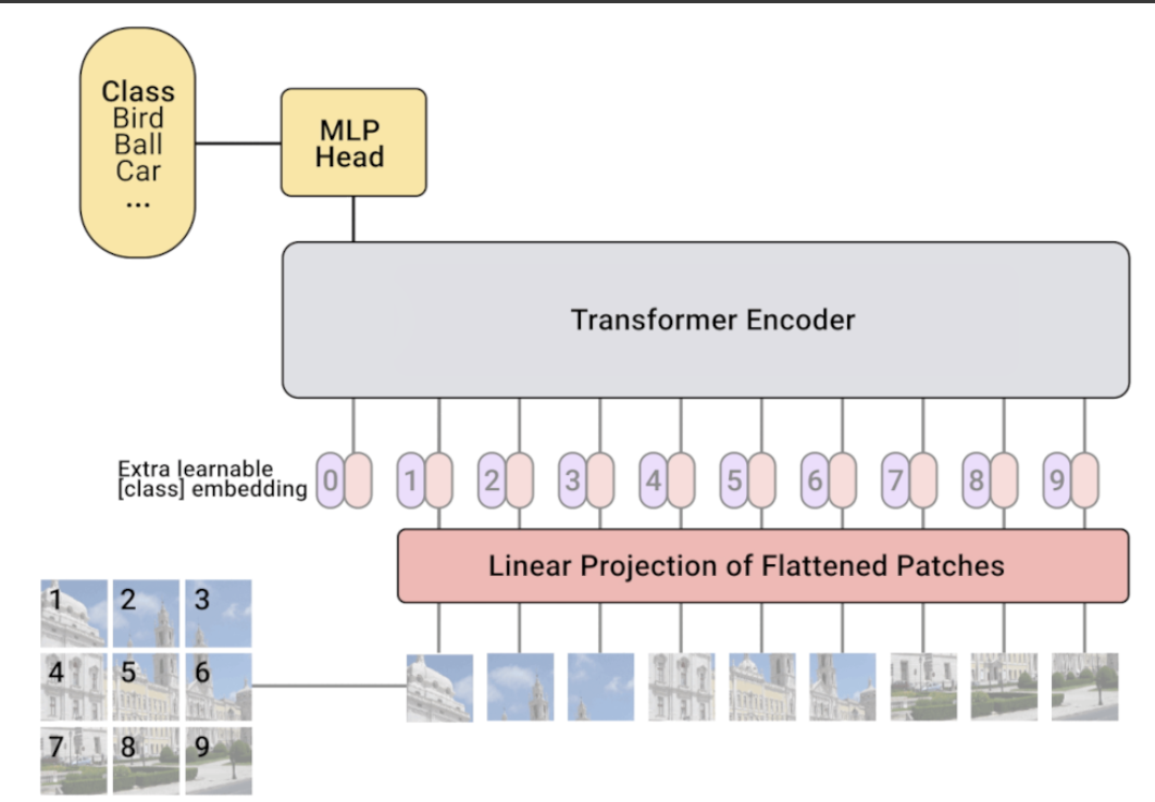
Let’s give an example of this:

• First step is to break the image into square patches, as recall earlier, we can treat these patches as sequential tokens, which transformers work well. These patches are flattened into a sequence of patches. Then, we apply a linear projection of the flattened patches, this is the same as when processing text data, we mapped the tokens of the input to their corresponding embeddings
• In these embeddings, we also want to encode the position into the embeddings, as the position in the sequence matters
• We then pass these embeddings into a transformer encoder
• Last, we pluck out the embeddings and pass it through an MLP (Dense NN), and then we use some classifier to predict the class of the image

Interesting Links

https://www.youtube.com/watch?v=kCc8FmEb1nY&t=0s&ab_channel=AndrejKarpathy