Graph Neural Networks — Overview
Graphs are prevalent in representing real-world objects and their connections. Graph Neural Networks (GNNs) have been developed to process graph data effectively, with significant advancements enhancing their capabilities. GNNs are now applied in diverse fields such as antibacterial discovery, physics simulations, fake news detection, traffic prediction, and recommendation systems. These applications leverage the expressive power of GNNs to analyze and make predictions based on the complex relationships within graph-structured data.
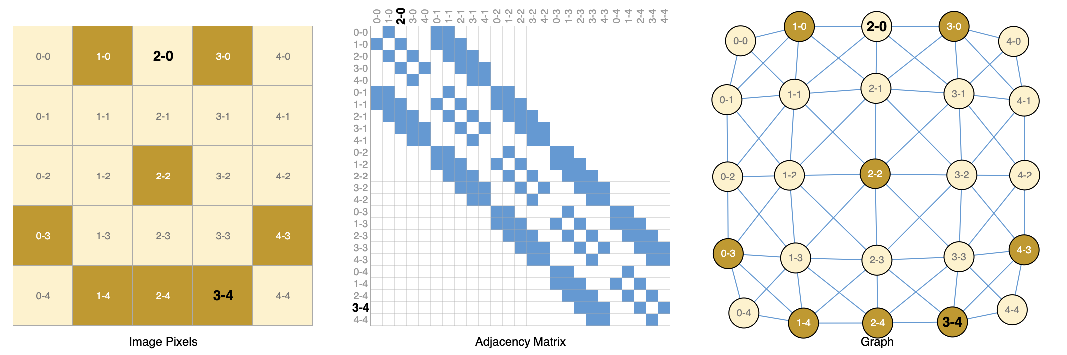
There are lots of data that take on the structure of graphs → computer networks, social networks, citation networks, etc. However, there are other data that can be expressed as graphs, that you may not have thought of. For example, images as graphs. We typically think of images as rectangular grids with image channels, representing them as arrays (e.g., 244x244x3 floats). Another way to think of images is as graphs with regular structure, where each pixel represents a node and is connected via an edge to adjacent pixels. Each non-border pixel has exactly 8 neighbours, and the information stored at each node is a 3-dimensional vector representing the RGB value of the pixel.
A way of visualizing the connectivity of a graph is through its adjacency matrix. We order the nodes, in this case each of 25 pixels in a simple 5x5 image of a smiley face, and fill a matrix of x with an entry if two nodes share an edge. Note that each of these three representations below are different views of the same piece of data.
We have described some examples of graphs in the wild, but what tasks do we want to perform on this data? There are three general types of prediction tasks on graphs: graph-level, node-level, and edge-level.
- In a graph-level task, we predict a single property for a whole graph.
- For example, for a molecule represented as a graph, we might want to predict what the molecule smells like, or whether it will bind to a receptor implicated in a disease.
- For a node-level task, we predict some property for each node in a graph.
- A classic example of a node-level prediction problem is Zach’s karate club. The nodes represent individual karate practitioners, and the edges represent interactions between these members outside of karate. The prediction problem is to classify whether a given member becomes loyal to either Mr. Hi or John H, after the feud.
- For an edge-level task, we want to predict the property or presence of edges in a graph.
- One example of edge-level inference is in image scene understanding. Beyond identifying objects in an image, deep learning models can be used to predict the relationship between them.
- For the three levels of prediction problems described above (graph-level, node-level, and edge-level), we will show that all of the following problems can be solved with a single model class, the GNN. But first, let’s take a tour through the three classes of graph prediction problems in more detail, and provide concrete examples of each.
The challenges of using graphs in machine learning
The main challenge, is representing graphs a tensors. In many situations, data structures like adjacency matrices work well. But, what about for representing arbitrary graphs? Often, this leads to very sparse adjacency matrices, which are space-inefficient. Consider the following representation for relationships between characters in Shakespeare’s Othello:
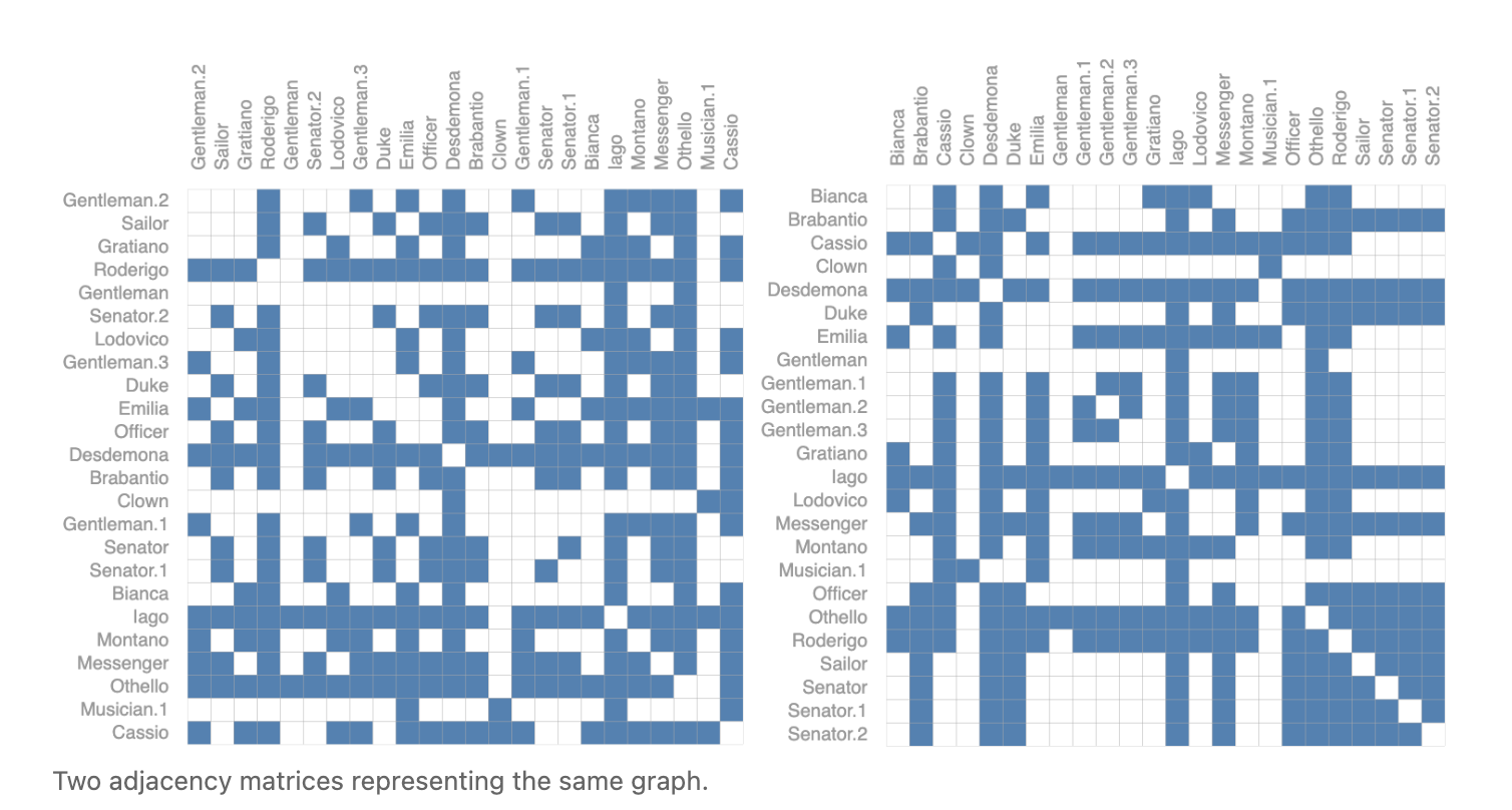
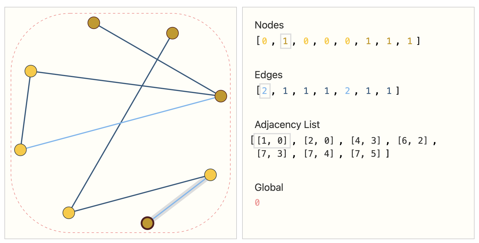
These are just 2. The total number of possible versions is untenable, as if we only had 4 nodes, we would already have 24 possible graphs. An elegant way and memory-efficient method is to use adjacency lists.
Now, let’s take a look at building a GNN:
Deeper into Graph NNs
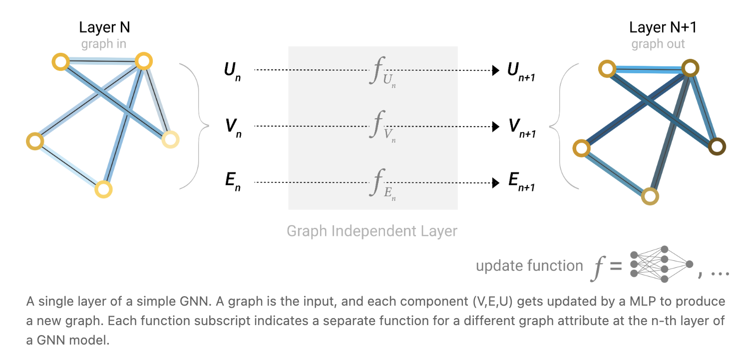
We will start with the simplest GNN architecture, one where we learn new embeddings for all graph attributes (nodes, edges, global), but where we do not yet use the connectivity of the graph. This GNN uses a separate multilayer perceptron (MLP) (or your favorite differentiable model) on each component of a graph; we call this a GNN layer. For each node vector, we apply the MLP and get back a learned node-vector. We do the same for each edge, learning a per-edge embedding, and also for the global-context vector, learning a single embedding for the entire graph.
As is common with neural networks modules or layers, we can stack these GNN layers together.
GNN Predictions by Pooling Information
We have built a simple GNN, but how do we make predictions in any of the tasks we described above? Let’s consider the simple example of binary classification. Say we want to make binary predictions on nodes, and the graph already contains node information, the approach is straightforward - for each embedding, apply a linear classifier.
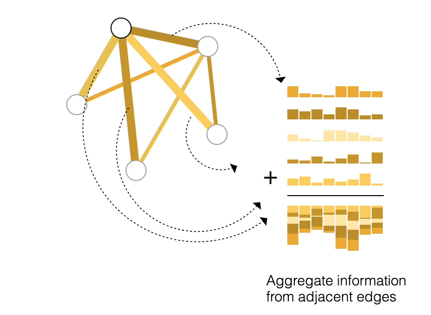
However, it is not always so simple. For instance, you might have information in the graph stored in edges, but no information in nodes, but still need to make predictions on nodes. We need a way to collect information from edges and give them to nodes for prediction. We can do this by pooling. Pooling proceeds in two steps:
- Gather each of their embeddings and concatenate them into a matrix
- The gathered embeddings are then aggregated, usually via a sum operation (think taking element-wise sum of the embeddings of node vector and all the adjacent edge vectors) The following is a good diagram of this:
So, if we only have edge-level features, and want to predict binary node information, we can use pooling to pass information to where it needs to go. The same applies if we only have node-level features, and are trying to predict binary edge-level information. Then, once we have these new embeddings, we just pass it through some classifier like a logistic regression or a multilayer-perceptron.
- The important, in this case, of the GNN is in computing the embeddings for all nodes/edges in the graph
The same is for predicting a binary global property → we gather all available node or edge information together and aggregate them → very similar to the pooling layers in CNNs. So, this is a simple idea on how to build a GNN, and make binary predictions by routing information between different parts of the graph. Note that in this simplest GNN formulation, we’re not using the connectivity of the graph at all inside the GNN layer. Each node is processed independently, as is each edge, as well as the global context. We only use connectivity when pooling information for prediction.
Passing messages between parts of the graph
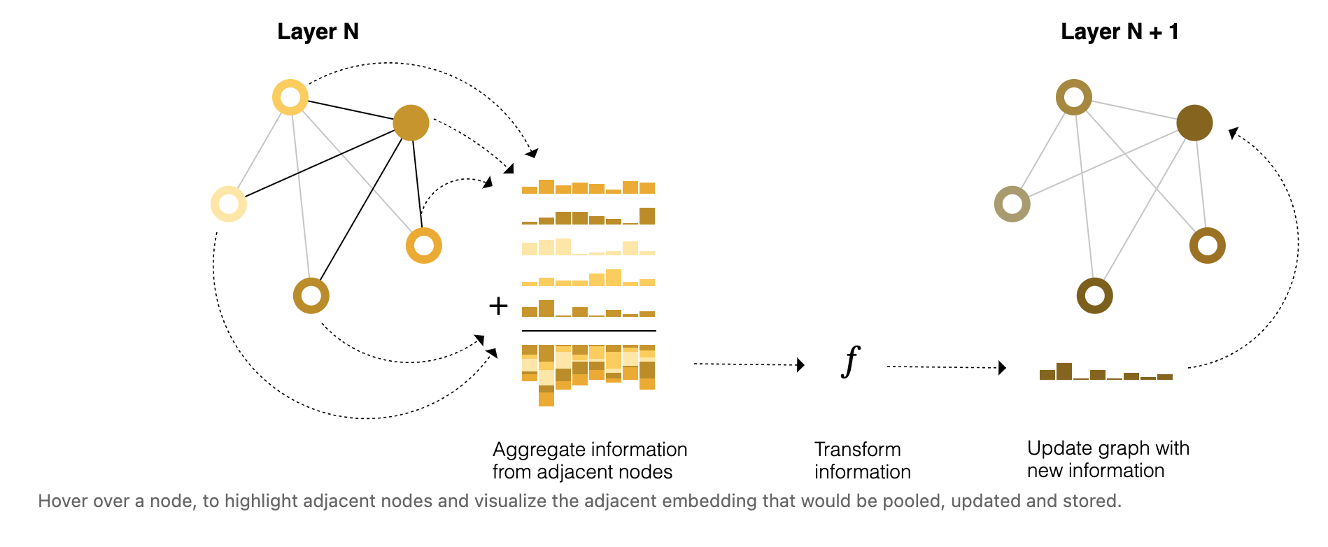
We could make more sophisticated predictions by using pooling within the GNN layer, in order to make our learned embeddings aware of graph connectivity. We can do this using message massing, where neighbouring nodes or edges exchange information and influence each other’s updated embeddings. 3 steps:
- For each node, gather all neighbouring node embeddings
- Aggregate all messages via an aggregate function (e.g sum)
- All pooled messages are passed through an update function → learned via NN
Just as pooling can be applied to either nodes or edges, message passing can occur between either nodes or edges.
 This is the simplest example of message-passing in a GNN layer. What’s interesting, is this is reminiscent of a standard convolution operation:
- Both are operations to aggregate and process the information of an element’s neighbours in order to update the elements value.
- In graphs, the element is a node and in images, the element is a pixel
- However, the number of neighbouring nodes in a graph can be variable, unlike in an image where each pixel has a set number of neighbouring elements.
By stacking message passing GNN layers together, a node can eventually incorporate information from across the entire graph: after three layers, a node has information about the nodes three steps away from it.
Learning edge representations
Our dataset does not always contain all types of information (node, edge, and global context). When we want to make a prediction on nodes, but our dataset only has edge information, we showed above how to use pooling to route information from edges to nodes, but only at the final prediction step of the model. We can share information between nodes and edges within the GNN layer using message passing.
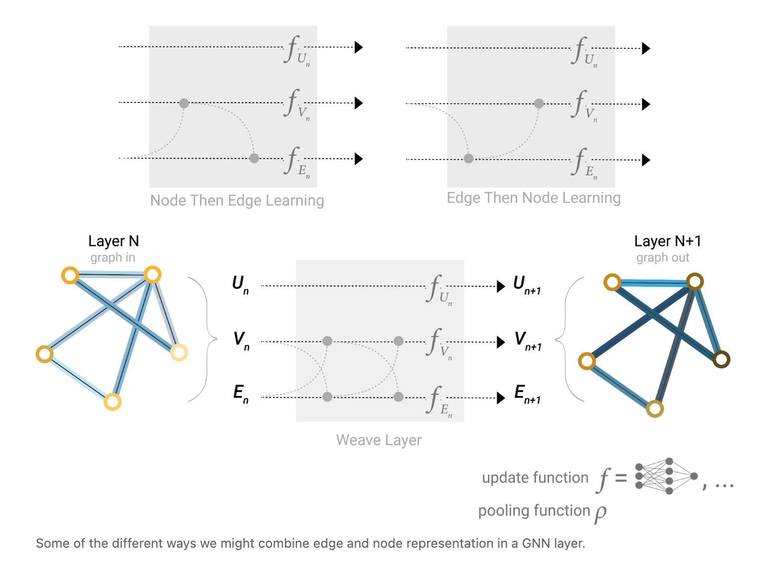
We can incorporate the information from neighbouring edges in the same way we used neighbouring node information earlier, by first pooling the edge information, transforming it with an update function, and storing it. However, the node and edge information stored in a graph are not necessarily the same size or shape, so it is not immediately clear how to combine them. One way is to learn a linear mapping from the space of edges to the space of nodes, and vice versa. A.K.A → Introduce some weight matrix to learn this mapping.
Which graph attributes we update and in which order we update them is one design decision when constructing GNNs. We could choose whether to update node embeddings before edge embeddings, or the other way around. This is an open area of research with a variety of solutions.
Learning global representations
There is one flaw with the networks we have described so far: nodes that are far away from each other in the graph may never be able to efficiently transfer information to one another, even if we apply message passing several times. For one node, If we have k-layers, information will propagate at most k-steps away.
- One solution would be to have all nodes be able to pass information to each other. Unfortunately for large graphs, this quickly becomes computationally expensive (although this approach, called ‘virtual edges’, has been used for small graphs such as molecules).
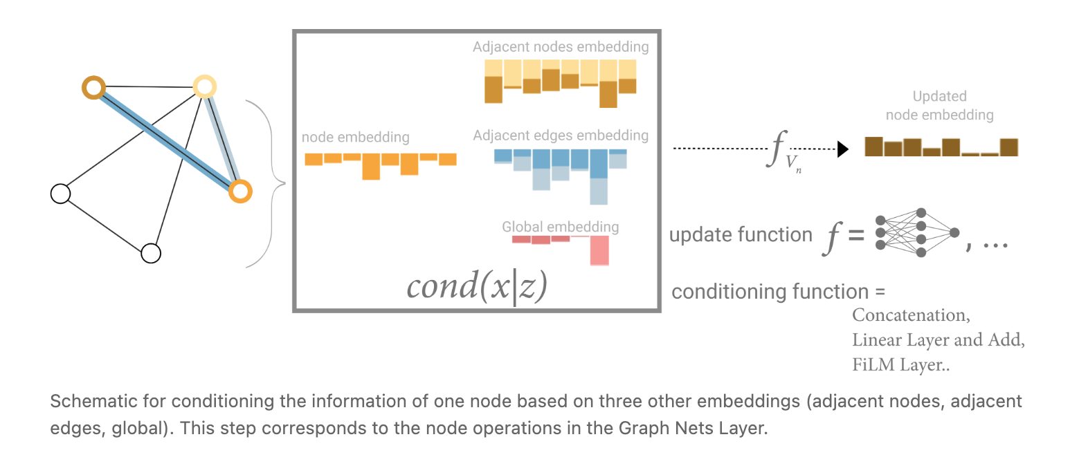
One solution to this problem is by using the global representation of a graph (U) which is sometimes called a master node. In this view all graph attributes have learned representations, so we can leverage them during pooling by conditioning the information of our attribute of interest with respect to the rest. For example, for one node we can consider information from neighbouring nodes, connected edges and the global information. To condition the new node embedding on all these possible sources of information, we can simply concatenate them. Additionally we may also map them to the same space via a linear map and add them or apply a feature-wise modulation layer, which can be considered a type of featurize-wise attention mechanism.
Please read the following (if have time, prob not, but some interesting things):