Chapter 7 - RNN'S and Transformer Architecture Part 1

Sequence data

Sequence data is very prevalent, classical examples include:

• Speech recognition
• Music genration
• Sentiment classification
• Machine translation
• Video activity recognition: sequence of frames → predict activity

Lot’s of different types of sequence problems. Let’s define a notation we’ll use to build these sequence models.

→ Motivating Example:

• $x$: Harry Potter and Hermione Granger invented a new spell
• $y$: One output per input word → target output tells us, for each of the input words, is that part of a person’s name
  • For the above: 1 1 0 1 1 0 0 0 0
• Let $x^{<i>}$ be the index position $i$ of the input $x$
• Let $y^{<i>}$ be the index into the output sequence
• In this example, length of input $T_x=T_y$ length of output → of course, not always the case

We’ve been using $X^{(i)}$ to denote the ith training sample → denote $X^{(i)<t>}$ to denote t-th index in the sequence of training sample i, and we let $T_x^{(i)}$ be the input sequence length for training sample i. The same notation applies for $y$. This is our first foray into NLP. First, we need a vocabulary/dictionary → a list of all words in our representation. This takes on the form of some high-dimension vector (~50k is common in commercial applications). Let’s consider a very small example of this, around 10k words in our dictionary, for illustrations purposes.

How do we obtain this? Can either look online for most common 10k words, or search our training data. Then, with this, we one-hot encode our input words. So, for example, “Harry” becomes → $[\mathrm{000...010...0}{]}^T$ is the representation, where entry is 1 at the index of “Harry” in the dictionary.

What if we encounter a word not in the dictionary? → Allocate a UNKOWN WORD in the dictionary

So, this has been a notation for our sequence data. Before we jump into the details of transformers, its important to look at their predecessor → RNN (Recurrent Neural Networks), to learn the mapping from $x$ to $y$

Recurrent Neural Networks

One option is to just build some standard dense neural network:

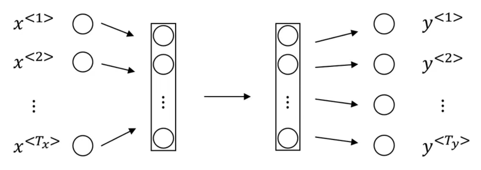
But, this does not work well:

• Firstly, the inputs and outputs can be different lengths in different examples.
• A naive neural network does not share features learned across different positions of text
  • e.g if the network learns that “Harry” appearing at position 1 correlates to some persons name, we want it to also associate “Harry” at index $j$ is also some persons name
  • This idea is similar to what we saw in CNN → things learned in one part of image can be generalized to other parts of the image

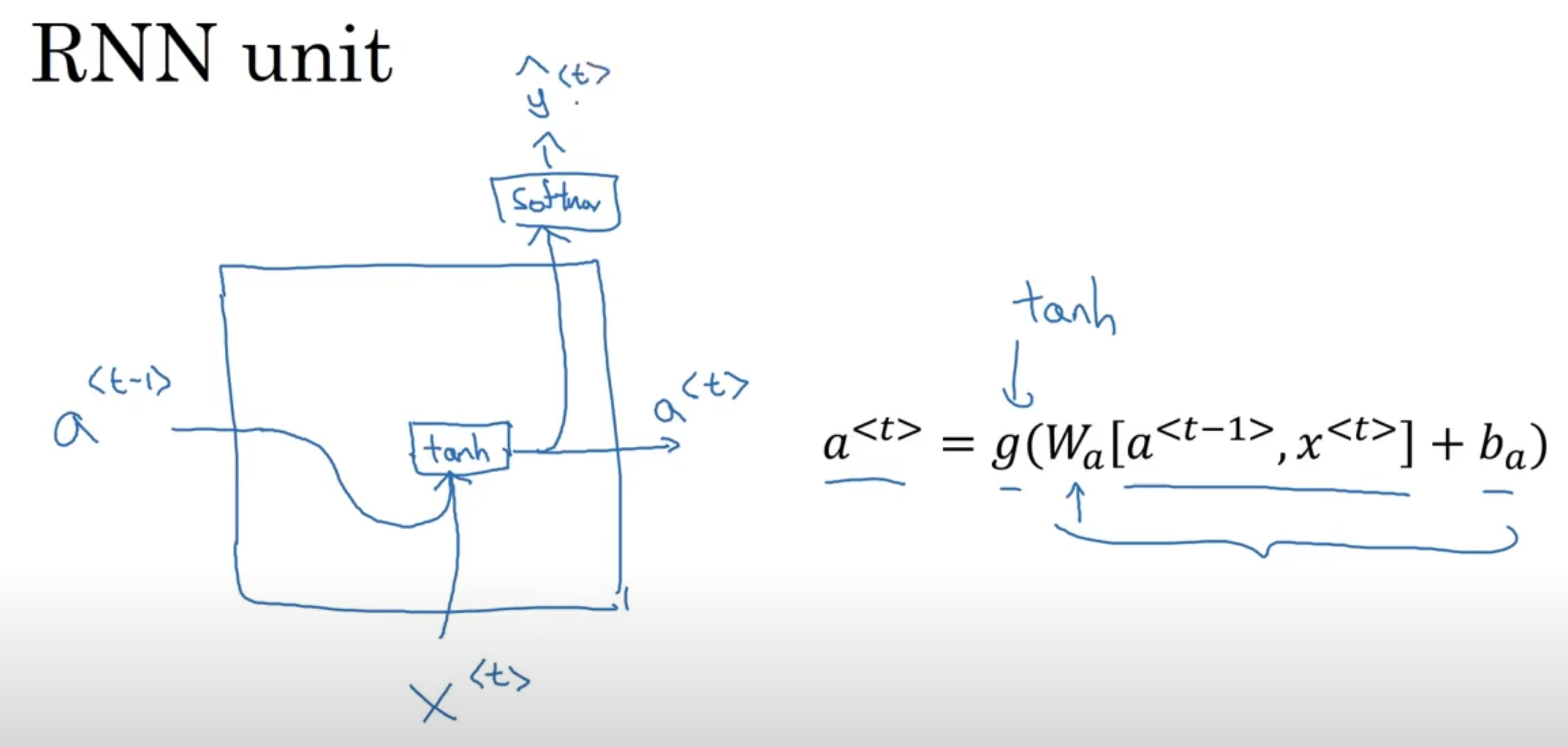
A RNN does not have either of these disadvantages. Let’s see how. → Overview So, reading the input from left to right, the first word read is $x^{<1>}$. Consider the following illustration:

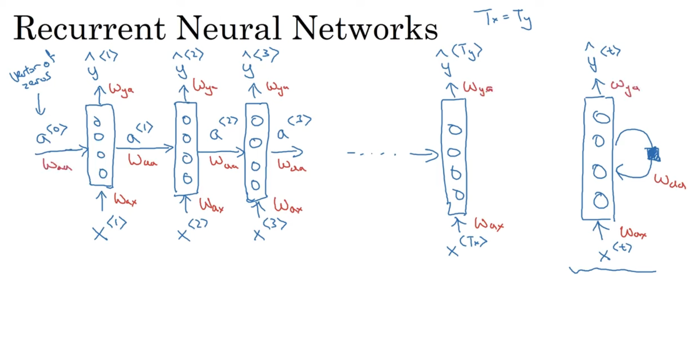We are reading left to right, and we know $x^{<1>}$ is the first word, and we feed it into a neural network layer. It will predict the output (is this word in a name or not). What an RNN does, is when it goes to read second word, instead of predicting only on $x^{<2>}$, it will also use the result of the earlier time-stamp, specifically, the activation of time-step 1: $a^{<1>}$. This continues until the very last time step. The RNN scans through the data, left to right, the parameter it uses for each time-step, are shared. The parameters governing the connection from $x^{<1>}$ to the layer, is the $W_{ax}$. Let’s see how these parameters work.

• One weakness of the RNN is it only uses earlier information to make a prediction (for y3, it uses x1, x2, x3, but not anything later). This can be a problem. Consider the statement “He said, Teddy Roosevelt was a great president”, where it would be useful to know about about the later parts of the sentence. What if we had “He said, Teddy bears are on sale!“? Given 3 words, impossible to tell whether it is name or not.
• This is the limitation of this architecture → only uses earlier information, but not later information

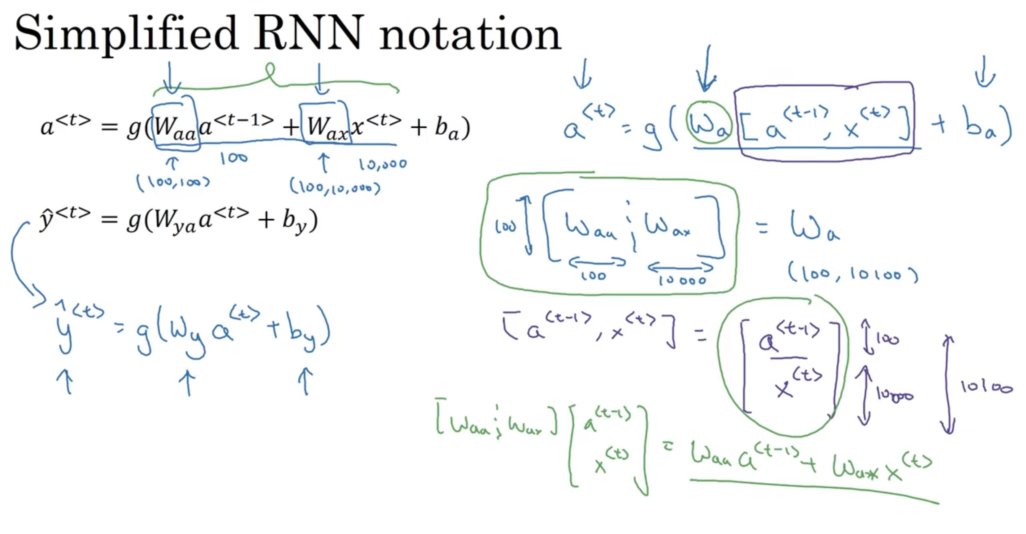
Let’s see the forward propagation for the above simple RNN → $a^{<1>}=g_1(W_{aa}{a}^{<0>}+W_{ax}{a}^{<1>}+b_a)$ and $\widehat{y^1}=g_2(W^{ya}{a}^{<1>}+b_y)$ where $g$ is our activation function. A quick thing on notation, when we refer to $W_{ax}$, the second index indicates this will be multiplied some x-like quantity, and the a means it will compute some a-like quantity. The most common activation function is often a $tanh$ in the choice of RNNs. Then, depending on the problem, if it is a classification, could be something like $sigmoid$ for y. So these equations define the forward propagation in the RNN, making our way from $a_0$ to $a_t$. We introduce a notation simplification:

Examples of RNN Architecture

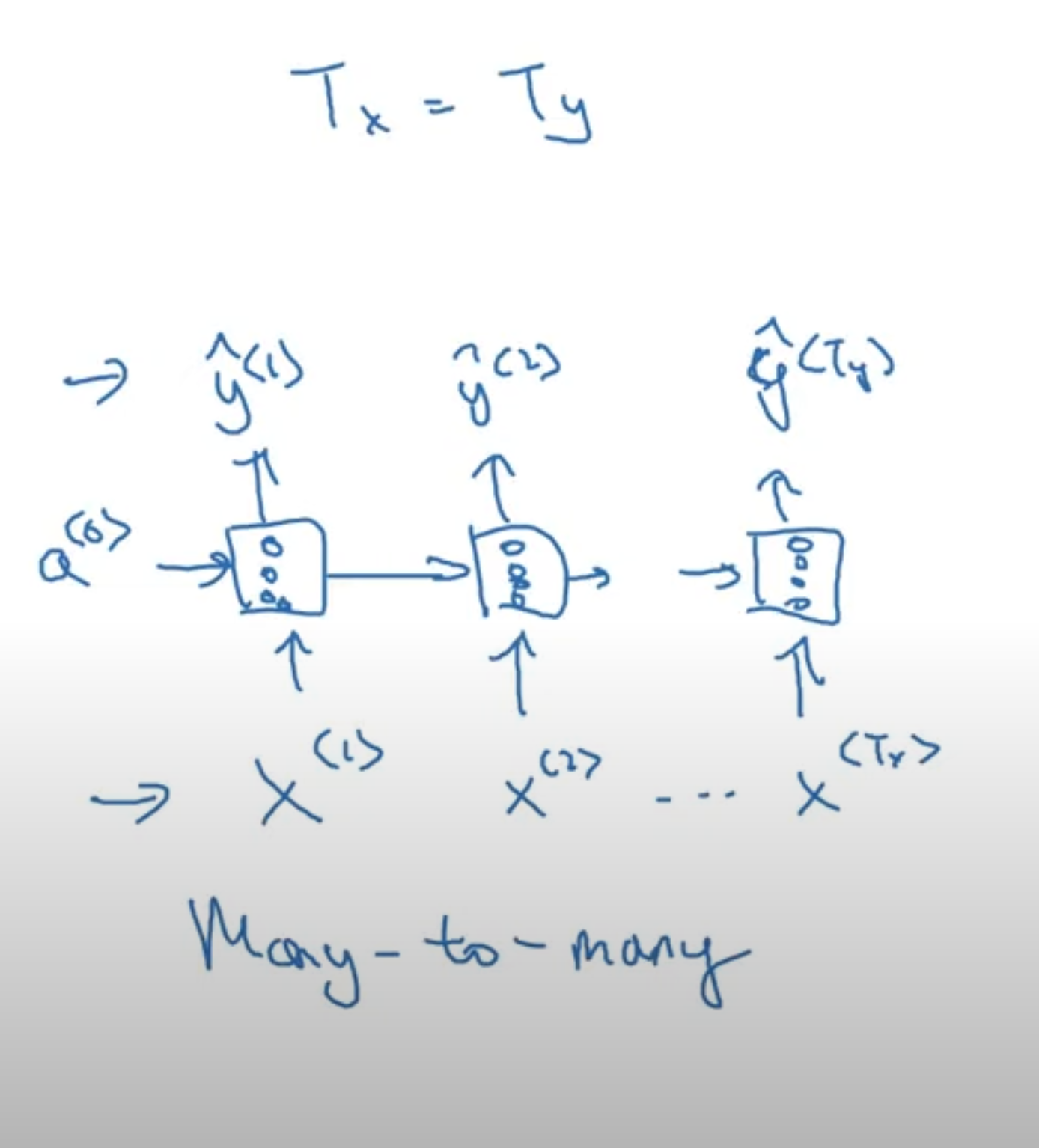
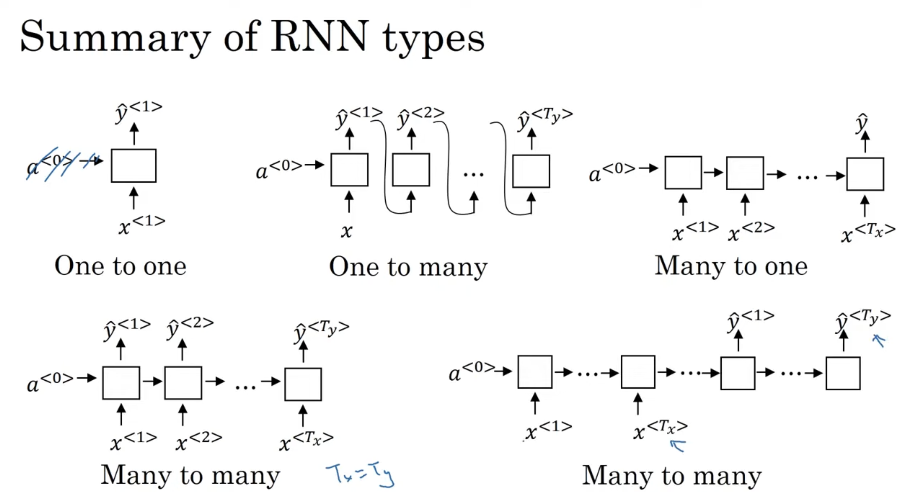
→ Many to Many That is, give a sequence data, we want to also predict some sequence. This is the RNN architecture we’ve seen so far:

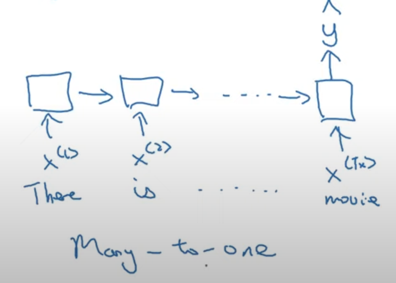
→ Many to One Say we wanted to use a RNN for movie review sentiment classification. The input $x$ would be something like “There is nothing to like in this movie”, and the label $y$ would be some binary value indicating positive or negative, or perhaps in the range from 1 to 5 indicating stars of rating. Regardless, the output of the model is one value.

→ Many to Many: Interesting Example An interesting example of the many to many architectures, is when the input and output sequence are different lengths. For an application like machine translation, the sentences translated would be different lengths. This is when we have an alternative RNN architecture:

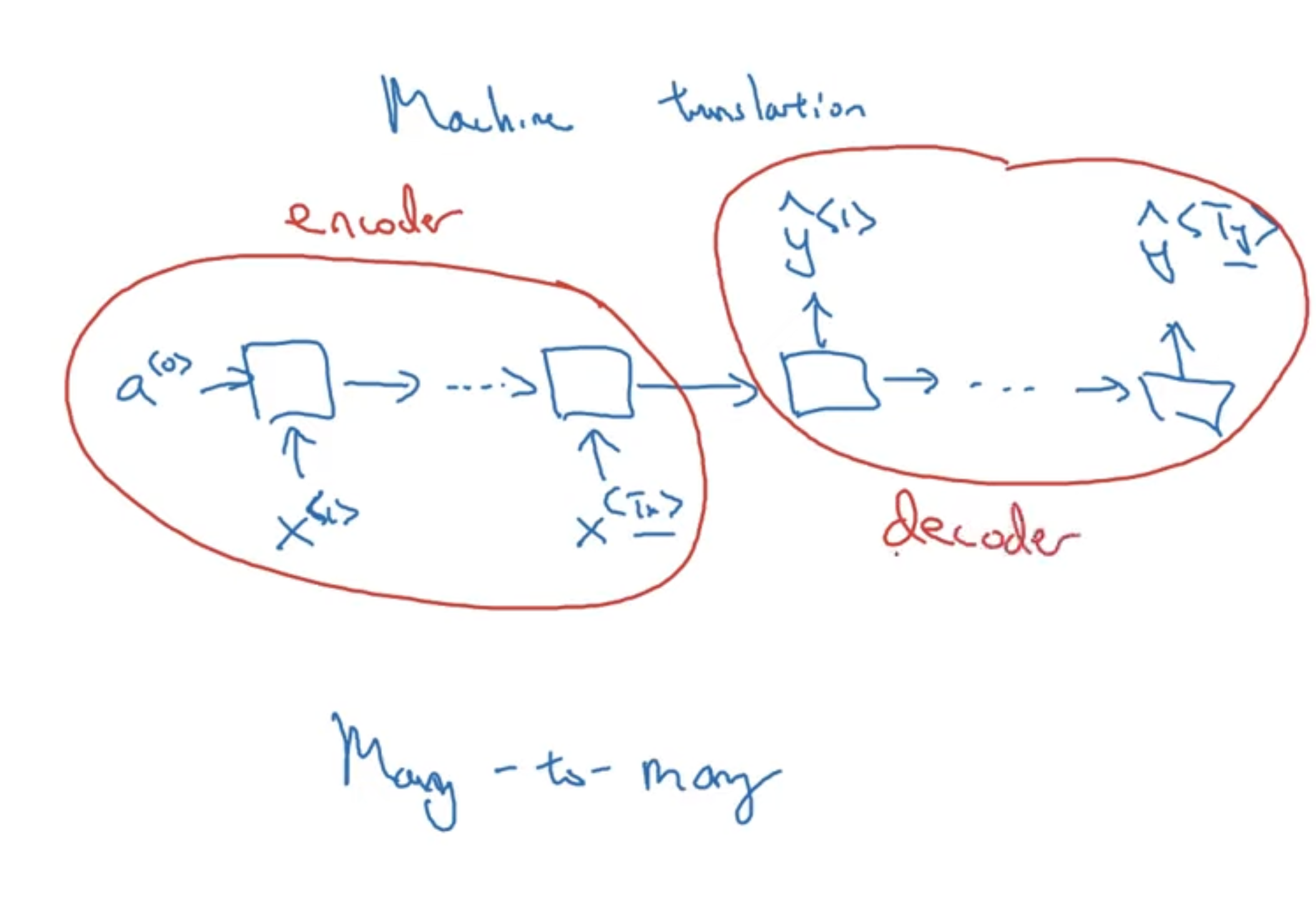
Now, we can have input and output sequences of different length. So, in this design, there are 2 distinct components of the RNN → encoder and decoder, which is similar to what we have in transformers, attention-based architectures.

So, these are the basic building blocks of RNN, and already, there are a wide range of models we can put together. But, there are some subtleties to sequence generation.

Language model and sequence generation

→ What is language modelling?

• Speech recognition:
  • The apple and pair salad
  • The apple and pear salad
  • Which one did I say?
    • Good system recognizes it is the second, where it computes:
    • P(The apple and pair salad) = $3.2\cdot 10^{-13}$
    • P(The apple and pear salad) = $5.7\cdot 10^{-10}$
    • So, the second one is much more likely, and be picked

Language modeling primarily involves predicting the next token (which could be a word, subword, or character) in a sequence of words. This task is central to many natural language processing (NLP) applications. The main idea is to create a probabilistic model that can predict the probability distribution of the next token given a sequence of previous tokens. This approach is fundamental to several key NLP tasks. The language model aims is to input a sentence, which we can represent as a sequence of outputs $y$, and estimates the probability of this sequence of words. So, how do we build one? Let’s see how do this with RNN. First, need large corpus (body, set) of english text. Given an input like “Cats average 15 hours of sleep a day”, where we tokenize this and one-hot encode them. We may also add a end of sentence token for some applications, and we will see some of this later.

→ RNN Model Example: Cats average 15 hours of sleep a day. <EOS>

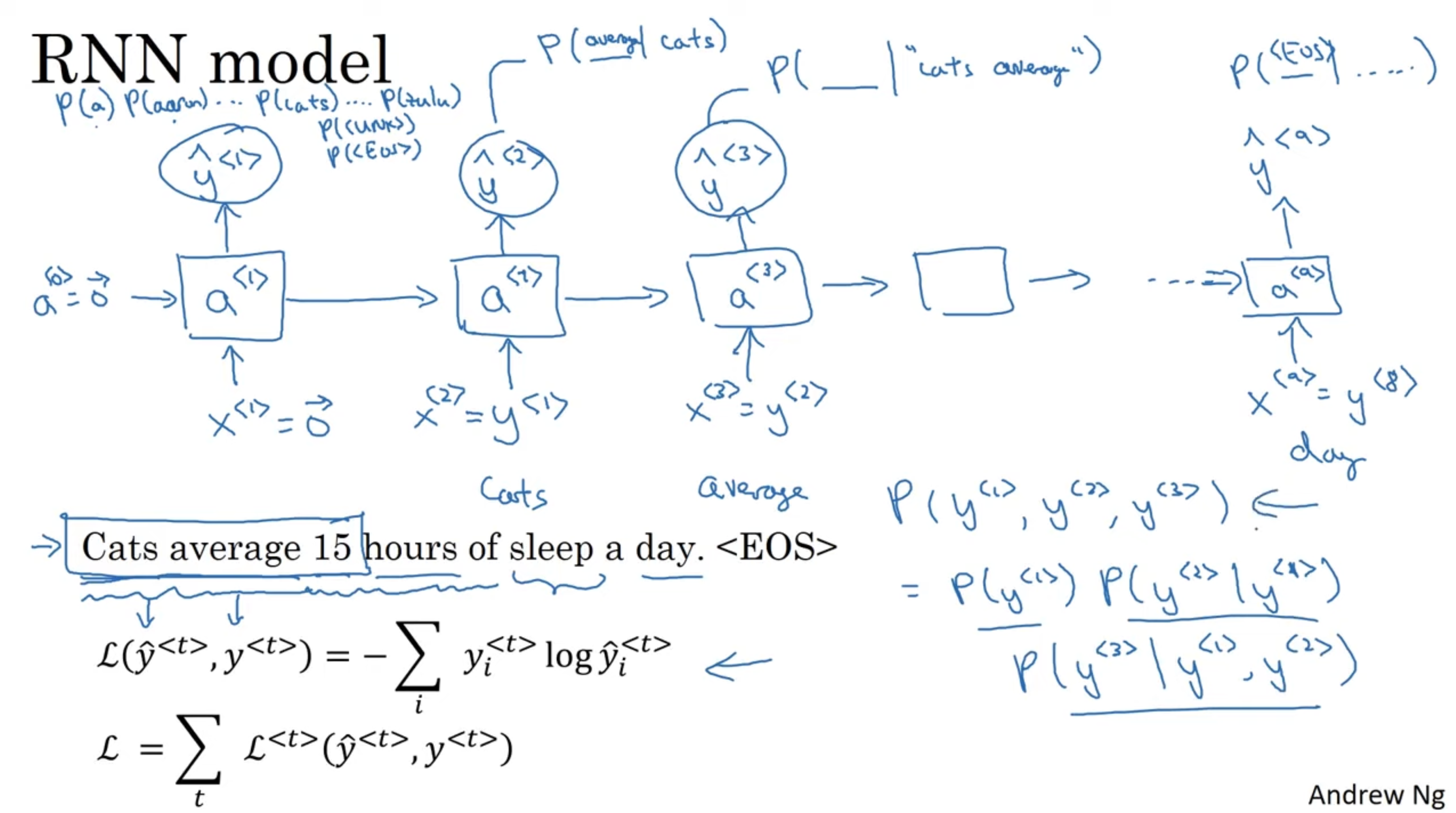The above defines a loss function for this, and illustrates the output of the RNN given this kind of sequence data. One of the challenges of training RNNs is the problem of vanishing gradient.

→ Vanishing gradients with RNNs The vanishing gradient problem is a common issue in training deep neural networks, particularly in networks with many layers, such as recurrent neural networks (RNNs) and deep feedforward networks. It occurs when the gradients of the loss function with respect to the model parameters become very small during back-propagation. This leads to extremely slow updates for the weights, which in turn hampers the learning process and makes it difficult for the model to converge to a good solution. This is shows itself in language processing as well.

Consider the following:

• The cat, which ate all the …, was full
• The cats, which ate all the …, were full

A characteristic about language, is that there often situations like this, where words that are far apart have large impact on the other. This distance is a short-coming of the RNN architecture we have seen so far. To explain why, recall that this is a problem in training deep neural networks as well, where we had some around ~100 layers. The issue is, the gradients computed for the later layers, would have a hard time back-propagating all the way back to the earlier layers to influence those weights. The same problem plagues our current RNN architecture. In addition english, these middle words can be arbitrarily long. Let’s see how to tackle this.

→ Gated Recurrent Unit This is a modification to the RNN hidden layers, that make it much better at capturing long range connections, and greatly reduces the vanishing gradient problem. We saw that we have activation function:

In a GRU unit, we introduce a new variable called a memory cell, and what it does, is it provides a bit of memory to remember, for example, whether the cat was singular or plural, so that when the network does reach much further, it can still remember this. So, we denote $c$ as a memory-cell and we denote the value of this at time-step $t$ to be $c^{<t>}=a^{<t>}$. At every time step, we will consider over-writing the value of the memory cell.

The important idea of GRU is the presence of a gate. In particular. we have a reset gate and an update gate. The reset gate determines how much of the previous information we need to forget, while the update gate determines how much of the new information to retain and how much of the old information to pass along to the next time step. Consider the following:

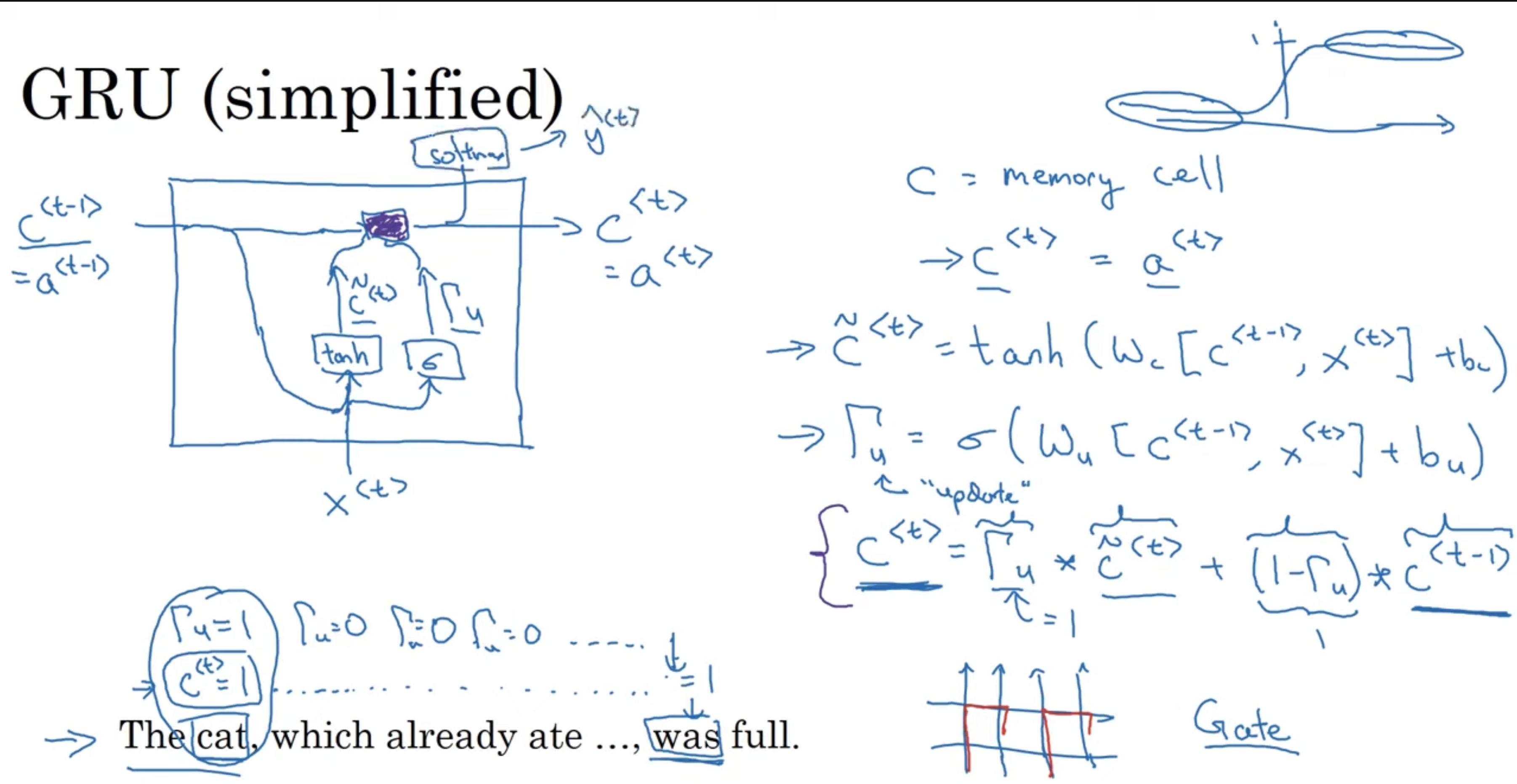
So, let’s see whats going on here. As mentioned above, we maintain a memory cell for each time-step, that remembers some information. First, we have tilde c, which is the value we may want to update our memory cell with. So, in the beginning of a sequence like “The cat, which already ate …, was full”, at “cat”, we set the memory cell to 1, to encode this information that the subject is a singular and not plural. Then, the rest of them, the gate should be 0, based on the gate function, which we illustrated above as sigmoid. While its not entirely a gate that maps to binary values, it is very close, and we can imagine it was a binary gate for better understand GRU.

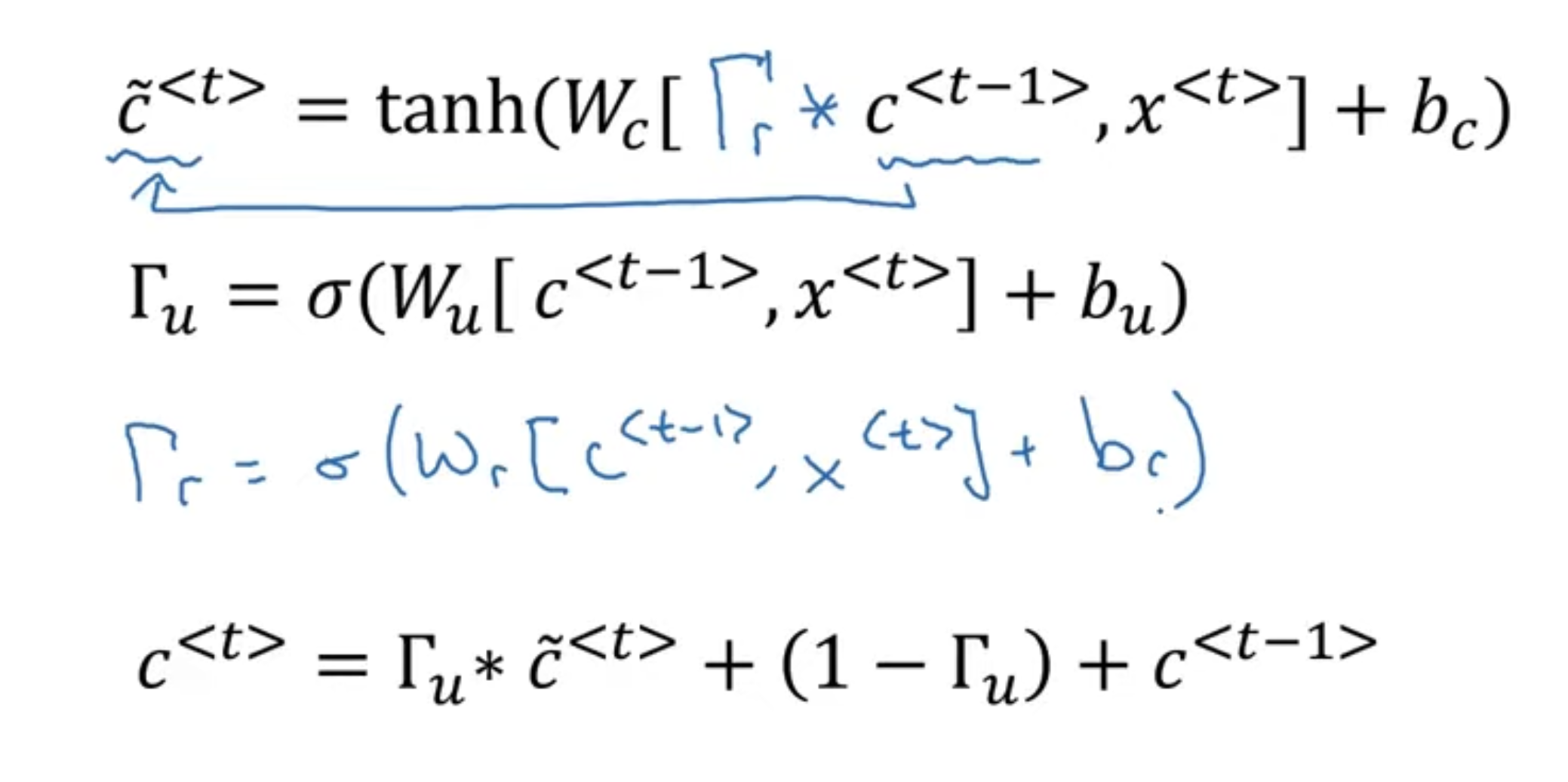
So, this gate should stay closed all the way until the end → so, information on singularity is maintained in the memory cell all the way until the end of sequence, helping to reduce issue of vanishing gradient. The above is a simplified version. What does the full GRU look like? We need to include an additional gate, called the reset gate. Essentially, it conveys us to how relevant the $c^{<t-1>}$ is to ${\tilde{c}}^{<t>}$:

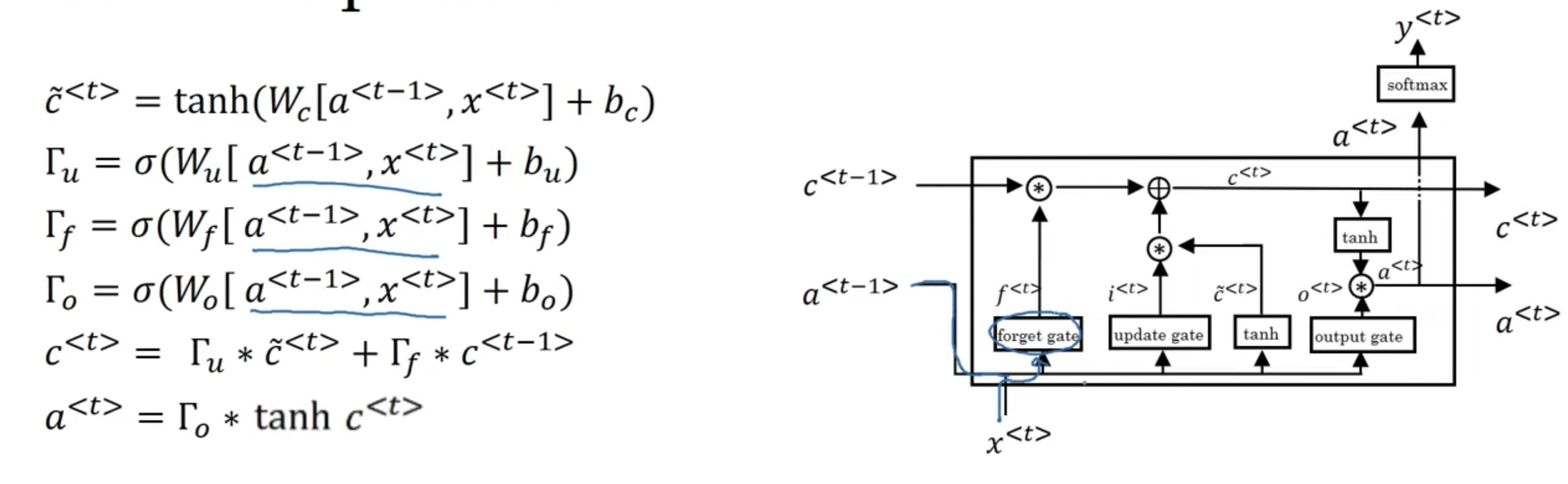
So, this was GRU. Another very common architecture, that serves a similar purpose to GRU, is LSTM (Long Short-term Memory). Here is a quick overview before we jump in: Architecture → LSTM (Long Short-Term Memory) Networks: • Components: LSTMs have three gates: the input gate, the forget gate, and the output gate, along with a cell state. • Gates: • Input Gate: Controls the extent to which new information flows into the cell state. • Forget Gate: Controls the extent to which information is retained or forgotten from the cell state. • Output Gate: Controls the extent to which the information from the cell state is used to compute the output. • Cell State: LSTMs maintain a cell state that runs through the entire sequence, allowing them to capture long-term dependencies.

→ GRU (Gated Recurrent Unit) Networks: • Components: GRUs have two gates: the reset gate and the update gate. • Gates: • Reset Gate: Determines how much of the previous state information to forget. • Update Gate: Determines how much of the new information to incorporate into the current state. • Simplified Architecture: GRUs combine the hidden state and cell state into a single state vector, simplifying the architecture compared to LSTMs.

→ Complexity • LSTMs: More complex due to having three gates and a separate cell state, which can capture more intricate temporal dynamics at the cost of increased computational complexity. • GRUs: Simpler due to having only two gates and a combined state vector, making them computationally more efficient and faster to train.

→ Performance • LSTMs: Often perform better on tasks requiring the learning of long-term dependencies because of their ability to control the flow of information more precisely with three gates. • GRUs: Perform comparably to LSTMs on many tasks but might be preferred when computational efficiency is critical. They tend to be faster to train and require less memory.

LSTM

This is largely the same ideas a GRU. Only difference is, it is more complex, as we introduce a third gate, and we move these out of the hidden layers (was concatenated on for GRU) into their own independent components:

So, this has been a general introduction to RNNs, and some of their most prevalent architectures. Recurrent neural networks were one approach to processing sequential data. In RNNs such as GRU and LSTM, data is processed sequentially, one time step at a time. This is what makes it difficult to parallelize computation, making this class of models expensive to train, especially for longer sequences. Likewise, while LSTM and GRU address the vanishing gradient problem, they can still struggle with extremely long-term dependencies to their sequential nature.

This gives rise to a new mechanism in addressing sequential data: attention. The transformer architecture was introduced in a paper by Google titled “Attention is All You Need”, address many of these limitations. Namely:

1. Attention Mechanism:
   1. Self-Attention: The core innovation of transformers is the self-attention mechanism, which allows the model to weigh the importance of different parts of the input sequence. This mechanism can relate different positions of a sequence directly, regardless of their distance.
   2. Parallel Processing: Unlike RNNs, transformers do not process data sequentially. They can process all positions of the sequence simultaneously, enabling parallel computation and significantly speeding up training.
2. Architecture:
   1. Encoder-Decoder: The original transformer model consists of an encoder and a decoder. The encoder processes the input sequence, while the decoder generates the output sequence, using attention mechanisms to focus on relevant parts of the input.
   2. Stacked Layers: Both the encoder and decoder are composed of multiple identical layers, each containing a multi-head self-attention mechanism and a feed-forward neural network.
3. Positional Encoding: Since transformers do not inherently handle sequential order, they use positional encodings to inject information about the position of each token in the sequence.

The evolution from RNNs to transformers marks a significant advancement in the field of machine learning, particularly in handling sequential data and enabling more powerful and efficient models for a wide range of applications. In the next lecture, we will see attention, and the way in which it handles sequential data.